

More on Technology

Frank Andrade
3 years ago
I discovered a bug that allowed me to use ChatGPT to successfully web scrape. Here's how it operates.
This method scrapes websites with ChatGPT (demo with Amazon and Twitter)

In a recent article, I demonstrated how to scrape websites using ChatGPT prompts like scrape website X using Python.
But that doesn’t always work.
After scraping dozens of websites with ChatGPT, I realized that simple prompts rarely work for web scraping.
Using ChatGPT and basic HTML, we can scrape any website.
First things first, use ChatGPT's advanced version (Playground)
ChatGPT Playground's enhanced version is needed to scrape websites quickly. It generates code faster and has less constraints.
Here’s how it looks.
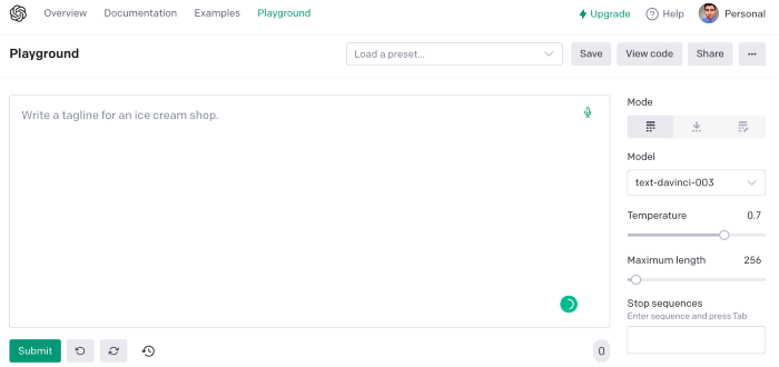
The classic ChatGPT display just allows you to type a prompt. Playground is more customizable and generates code faster than the basic version.
No more delays or restrictions.
In this tutorial, we'll write prompts underneath Playground.
How to Use ChatGPT to Scrape Any Website
To show you how to utilize ChatGPT to scrape any website, we'll use subslikescript, which lists movies.
Later in this post, I'll show you how to scrape Amazon and Twitter, but let's start easy.
If we try a basic prompt like “scrape the movie titles on this website: https://subslikescript.com/movies” it won’t scrape anything. Here’s when we need some HTML knowledge to build the right prompt for ChatGPT.Let's scrape the above movie titles. First, check the webpage. Right-click any element and choose Inspect.
Then see below.
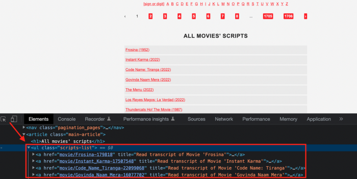
We identify the element to scrape (those in the red box). The data elements are ul, a, and scripts-list.
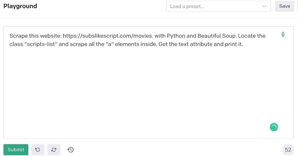
Here's the prompt for movie titles.
Scrape this website: https://subslikescript.com/movies with Python and Beautiful Soup. Locate the element with tag “ul” and class “scripts-list”. Scrape all the “a” elements inside. Get the text attribute and print it.
Code generated:
import requests
from bs4 import BeautifulSoup
page = requests.get('https://subslikescript.com/movies/')
soup = BeautifulSoup(page.content, 'html.parser')
scripts_list = soup.find(class_="scripts-list")
all_a_elements = scripts_list.find_all('a')
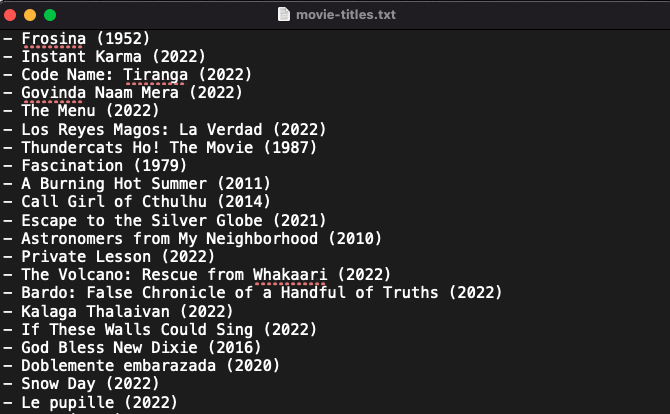
for element in all_a_elements:
print(element.get_text())It extracts movie titles successfully.
Let's scrape Amazon and Twitter.
ChatGPT's Amazon scraping
Consider scraping Amazon for self-help books. First, copy the Amazon link for self-help books.
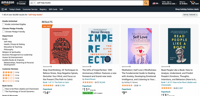
Here’s the link I got. Location-dependent connection. Use my link to replicate my results.
Now we'll check book titles. Here's our element.
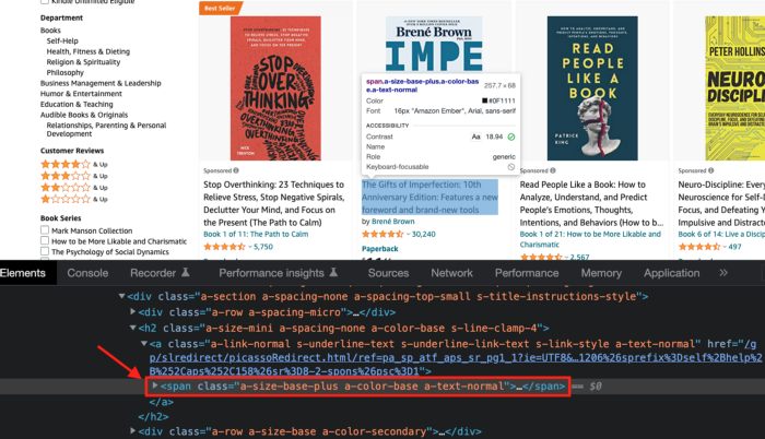
If we want to extract the book titles, we need to use the tag name span, class attribute name and a-size-base-plus a-color-base a-text-normalattribute value.
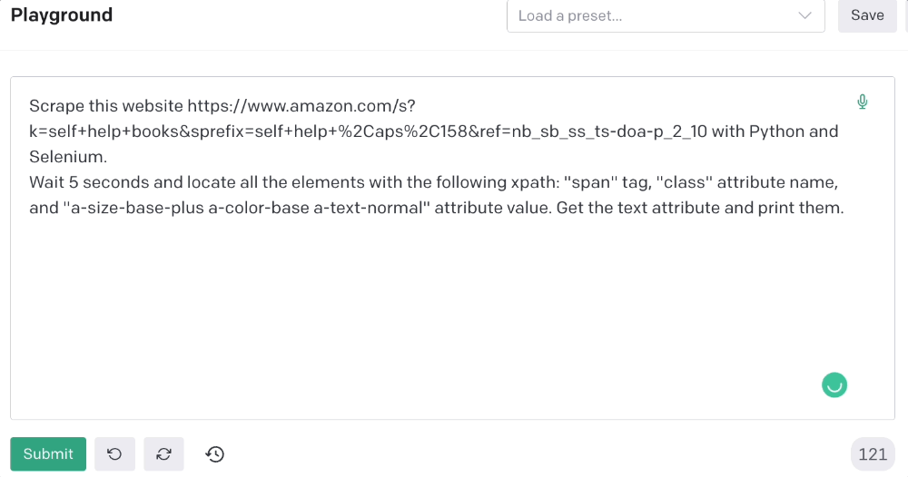
This time I'll use Selenium. I'll add Selenium-specific commands like wait 5 seconds and generate an XPath.
Scrape this website https://www.amazon.com/s?k=self+help+books&sprefix=self+help+%2Caps%2C158&ref=nb_sb_ss_ts-doa-p_2_10 with Python and Selenium.
Wait 5 seconds and locate all the elements with the following xpath: “span” tag, “class” attribute name, and “a-size-base-plus a-color-base a-text-normal” attribute value. Get the text attribute and print them.
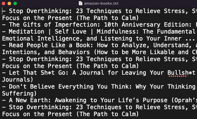
Code generated: (I only had to manually add the path where my chromedriver is located).
from selenium import webdriver
from selenium.webdriver.common.by import By
from time import sleep

#initialize webdriver
driver = webdriver.Chrome('<add path of your chromedriver>')

#navigate to the website
driver.get("https://www.amazon.com/s?k=self+help+books&sprefix=self+help+%2Caps%2C158&ref=nb_sb_ss_ts-doa-p_2_10")

#wait 5 seconds to let the page load
sleep(5)

#locate all the elements with the following xpath
elements = driver.find_elements(By.XPATH, '//span[@class="a-size-base-plus a-color-base a-text-normal"]')

#get the text attribute of each element and print it
for element in elements:
    print(element.text)

#close the webdriver
driver.close()
It pulls Amazon book titles.
Utilizing ChatGPT to scrape Twitter
Say you wish to scrape ChatGPT tweets. Search Twitter for ChatGPT and copy the URL.
Here’s the link I got. We must check every tweet. Here's our element.
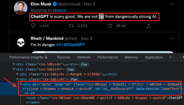
To extract a tweet, use the div tag and lang attribute.
Again, Selenium.
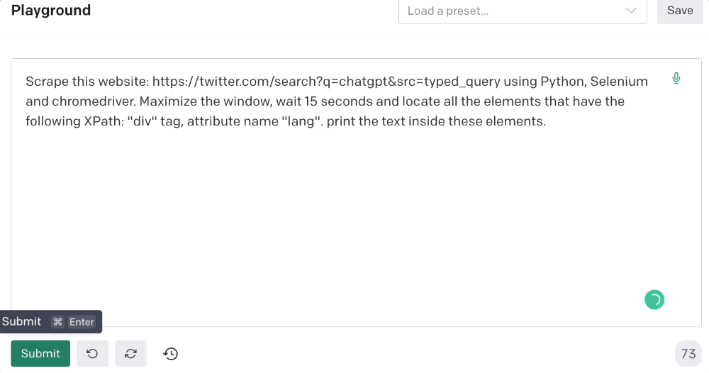
Scrape this website: https://twitter.com/search?q=chatgpt&src=typed_query using Python, Selenium and chromedriver.
Maximize the window, wait 15 seconds and locate all the elements that have the following XPath: “div” tag, attribute name “lang”. Print the text inside these elements.
Code generated: (again, I had to add the path where my chromedriver is located)
from selenium import webdriver
import time

driver = webdriver.Chrome("/Users/frankandrade/Downloads/chromedriver")
driver.maximize_window()
driver.get("https://twitter.com/search?q=chatgpt&src=typed_query")
time.sleep(15)

elements = driver.find_elements_by_xpath("//div[@lang]")
for element in elements:
    print(element.text)

driver.quit()
You'll get the first 2 or 3 tweets from a search. To scrape additional tweets, click X times.
Congratulations! You scraped websites without coding by using ChatGPT.

Ossiana Tepfenhart
3 years ago
Has anyone noticed what an absolute shitshow LinkedIn is?
After viewing its insanity, I had to leave this platform.
I joined LinkedIn recently. That's how I aim to increase my readership and gain recognition. LinkedIn's premise appealed to me: a Facebook-like platform for professional networking.
I don't use Facebook since it's full of propaganda. It seems like a professional, apolitical space, right?
I expected people to:
be more formal and respectful than on Facebook.
Talk about the inclusiveness of the workplace. Studies consistently demonstrate that inclusive, progressive workplaces outperform those that adhere to established practices.
Talk about business in their industry. Yep. I wanted to read articles with advice on how to write better and reach a wider audience.
Oh, sh*t. I hadn't anticipated that.

After posting and reading about inclusivity and pro-choice, I was startled by how many professionals acted unprofessionally. I've seen:
Men have approached me in the DMs in a really aggressive manner. Yikes. huge yikes Not at all professional.
I've heard pro-choice women referred to as infant killers by many people. If I were the CEO of a company and I witnessed one of my employees acting that poorly, I would immediately fire them.
Many posts are anti-LGBTQIA+, as I've noticed. a lot, like, a lot. Some are subtly stating that the world doesn't need to know, while others are openly making fun of transgender persons like myself.
Several medical professionals were posting explicitly racist comments. Even if you are as white as a sheet like me, you should be alarmed by this. Who's to guarantee a patient who is black won't unintentionally die?
I won't even get into how many men in STEM I observed pushing for the exclusion of women from their fields. I shouldn't be surprised considering the majority of those men I've encountered have a passionate dislike for women, but goddamn, dude.
Many people appear entirely too at ease displaying their bigotry on their professional profiles.

As a white female, I'm always shocked by people's open hostility. Professional environments are very important.
I don't know if this is still true (people seem too politicized to care), but if I heard many of these statements in person, I'd suppose they feel ashamed. Really.
Are you not ashamed of being so mean? Are you so weak that competing with others terrifies you? Isn't this embarrassing?
LinkedIn isn't great at censoring offensive comments. These people aren't getting warnings. So they were safe while others were unsafe.
The CEO in me would want to know if I had placed a bigot on my staff.

I always wondered if people's employers knew about their online behavior. If they know how horrible they appear, they don't care.
As a manager, I was picky about hiring. Obviously. In most industries, it costs $1,000 or more to hire a full-time employee, so be sure it pays off.
Companies that embrace diversity and tolerance (and are intolerant of intolerance) are more profitable, likely to recruit top personnel, and successful.
People avoid businesses that alienate them. That's why I don't eat at Chic-Fil-A and why folks avoid MyPillow. Being inclusive is good business.
CEOs are harmed by online bigots. Image is an issue. If you're a business owner, you can fire staff who don't help you.
On the one hand, I'm delighted it makes it simpler to identify those with whom not to do business.

Don’t get me wrong. I'm glad I know who to avoid when hiring, getting references, or searching for a job. When people are bad, it saves me time.
What's up with professionalism?
Really. I need to know. I've crossed the boundary between acceptable and unacceptable behavior, but never on a professional platform. I got in trouble for not wearing bras even though it's not part of my gender expression.
If I behaved like that at my last two office jobs, my supervisors would have fired me immediately. Some of the behavior I've seen is so outrageous, I can't believe these people have employment. Some are even leaders.
Like…how? Is hatred now normalized?
Please pay attention whether you're seeking for a job or even simply a side gig.
Do not add to the tragedy that LinkedIn comments can be, or at least don't make uninformed comments. Even if you weren't banned, the site may still bite you.
Recruiters can and do look at your activity. Your writing goes on your résumé. The wrong comment might lose you a job.
Recruiters and CEOs might reject candidates whose principles contradict with their corporate culture. Bigotry will get you banned from many companies, especially if others report you.
If you want a high-paying job, avoid being a LinkedIn asshole. People care even if you think no one does. Before speaking, ponder. Is this how you want to be perceived?
Better advice:
If your politics might turn off an employer, stop posting about them online and ask yourself why you hold such objectionable ideas.

Paul DelSignore
2 years ago
The stunning new free AI image tool is called Leonardo AI.
Leonardo—The New Midjourney?
Users are comparing the new cowboy to Midjourney.
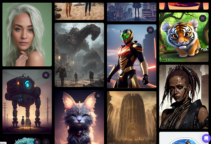
Leonardo.AI creates great photographs and has several unique capabilities I haven't seen in other AI image systems.
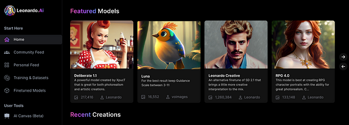
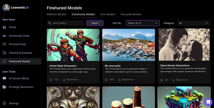
Midjourney's quality photographs are evident in the community feed.
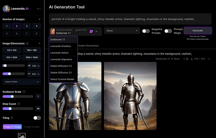
Create Pictures Using Models
You can make graphics using platform models when you first enter the app (website):
Luma, Leonardo creative, Deliberate 1.1.
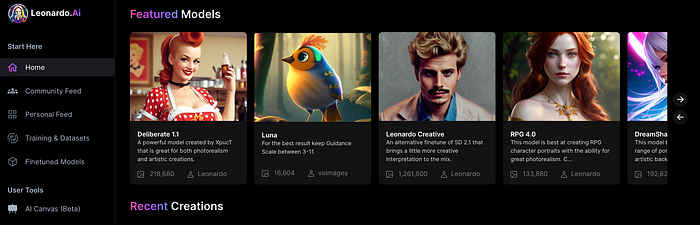
Clicking a model displays its description and samples:
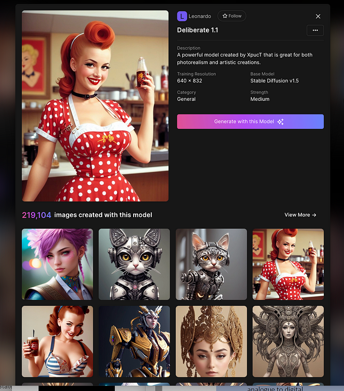
Click Generate With This Model.
Then you can add your prompt, alter models, photos, sizes, and guide scale in a sleek UI.
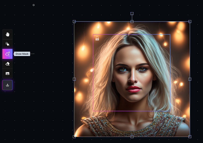
Changing Pictures
Leonardo's Canvas editor lets you change created images by hovering over them:
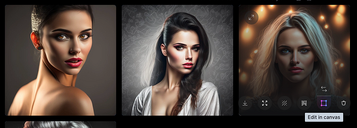
The editor opens with masking, erasing, and picture download.
Develop Your Own Models
I've never seen anything like Leonardo's model training feature.
Upload a handful of similar photographs and save them as a model for future images. Share your model with the community.
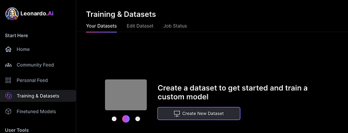
You can make photos using your own model and a community-shared set of fine-tuned models:
Obtain Leonardo access
Leonardo is currently free.
Visit Leonardo.ai and click "Get Early Access" to receive access.
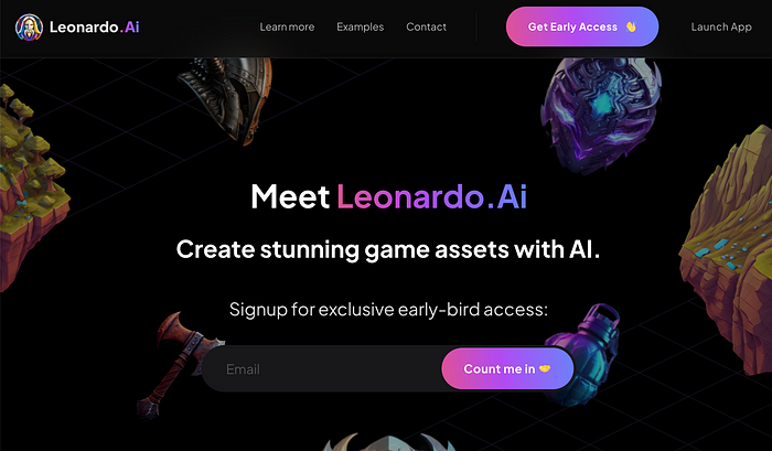
Add your email to receive a link to join the discord channel. Simply describe yourself and fill out a form to join the discord channel.
Please go to 👑│introductions to make an introduction and ✨│priority-early-access will be unlocked, you must fill out a form and in 24 hours or a little more (due to demand), the invitation will be sent to you by email.
I got access in two hours, so hopefully you can too.
Last Words
I know there are many AI generative platforms, some free and some expensive, but Midjourney produces the most artistically stunning images and art.
Leonardo is the closest I've seen to Midjourney, but Midjourney is still the leader.
It's free now.
Leonardo's fine-tuned model selections, model creation, image manipulation, and output speed and quality make it a great AI image toolbox addition.
You might also like

Darius Foroux
2 years ago
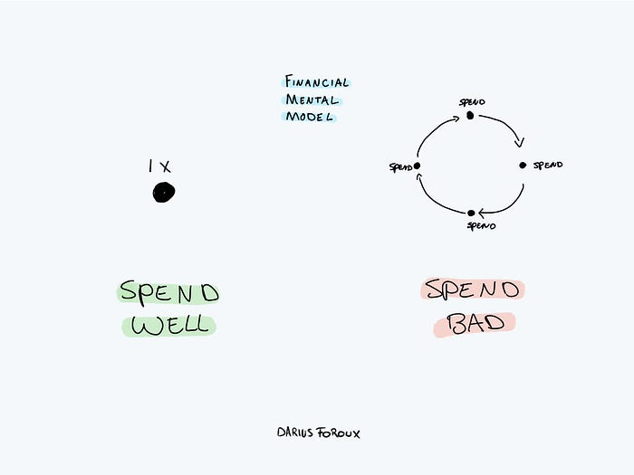
My financial life was changed by a single, straightforward mental model.
Prioritize big-ticket purchases
I've made several spending blunders. I get sick thinking about how much money I spent.
My financial mental model was poor back then.
Stoicism and mindfulness keep me from attaching to those feelings. It still hurts.
Until four or five years ago, I bought a new winter jacket every year.
Ten years ago, I spent twice as much. Now that I have a fantastic, warm winter parka, I don't even consider acquiring another one. No more spending. I'm not looking for jackets either.
Saving time and money by spending well is my thinking paradigm.
The philosophy is expressed in most languages. Cheap is expensive in the Netherlands. This applies beyond shopping.
In this essay, I will offer three examples of how this mental paradigm transformed my financial life.
Publishing books
In 2015, I presented and positioned my first book poorly.
I called the book Huge Life Success and made a funny Canva cover in 30 minutes. This:

That looks nothing like my present books. No logo or style. The book felt amateurish.
The book started bothering me a few weeks after publication. The advice was good, but it didn't appear professional. I studied the book business extensively.
I created a style for all my designs. Branding. Win Your Inner Wars was reissued a year later.
Title, cover, and description changed. Rearranging the chapters improved readability.
Seven years later, the book sells hundreds of copies a month. That taught me a lot.
Rushing to finish a project is enticing. Send it and move forward.
Avoid rushing everything. Relax. Develop your projects. Perform well. Perform the job well.
My first novel was underfunded and underworked. A bad book arrived. I then invested time and money in writing the greatest book I could.
That book still sells.
Traveling
I hate travel. Airports, flights, trains, and lines irritate me.
But, I enjoy traveling to beautiful areas.
I do it strangely. I make up travel rules. I never go to airports in summer. I hate being near airports on holidays. Unworthy.
No vacation packages for me. Those airline packages with a flight, shuttle, and hotel. I've had enough.
I try to avoid crowds and popular spots. July Paris? Nuts and bolts, please. Christmas in NYC? No, please keep me sane.
I fly business class behind. I accept upgrades upon check-in. I prefer driving. I drove from the Netherlands to southern Spain.
Thankfully, no lines. What if travel costs more? Thus? I enjoy it from the start. I start traveling then.
I rarely travel since I'm so difficult. One great excursion beats several average ones.
Personal effectiveness
New apps, tools, and strategies intrigue most productivity professionals.
No.
I researched years ago. I spent years investigating productivity in university.
I bought books, courses, applications, and tools. It was expensive and time-consuming.
Im finished. Productivity no longer costs me time or money. OK. I worked on it once and now follow my strategy.
I avoid new programs and systems. My stuff works. Why change winners?
Spending wisely saves time and money.
Spending wisely means spending once. Many people ignore productivity. It's understudied. No classes.
Some assume reading a few articles or a book is enough. Productivity is personal. You need a personal system.
Time invested is one-time. You can trust your system for life once you find it.
Concentrate on the expensive choices.
Life's short. Saving money quickly is enticing.
Spend less on groceries today. True. That won't fix your finances.
Adopt a lifestyle that makes you affluent over time. Consider major choices.
Are they causing long-term poverty? Are you richer?
Leasing cars comes to mind. The automobile costs a fortune today. The premium could accomplish a million nice things.
Focusing on important decisions makes life easier. Consider your future. You want to improve next year.

Navdeep Yadav
3 years ago
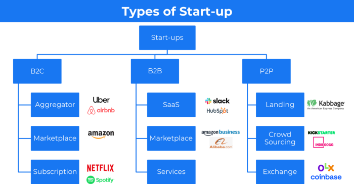
31 startup company models (with examples)
Many people find the internet's various business models bewildering.
This article summarizes 31 startup e-books.
1. Using the freemium business model (free plus premium),
The freemium business model offers basic software, games, or services for free and charges for enhancements.
Examples include Slack, iCloud, and Google Drive
Provide a rudimentary, free version of your product or service to users.
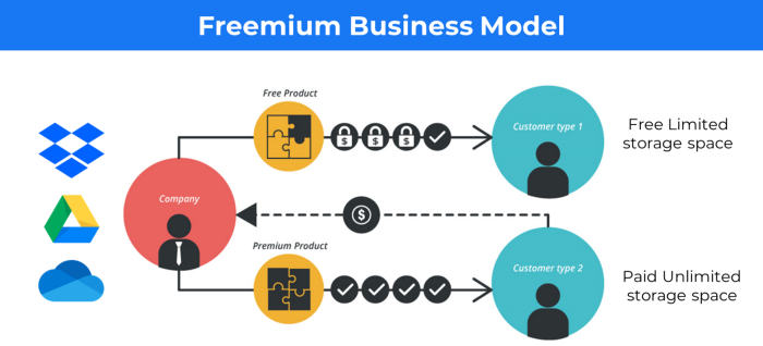
Google Drive and Dropbox offer 15GB and 2GB of free space but charge for more.
Freemium business model details (Click here)
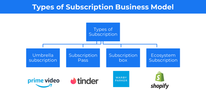
2. The Business Model of Subscription
Subscription business models sell a product or service for recurring monthly or yearly revenue.
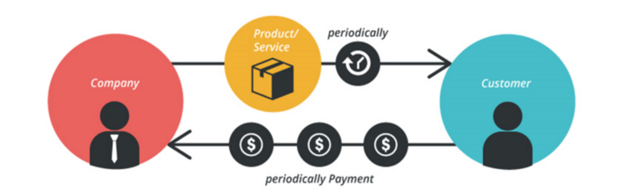
Examples: Tinder, Netflix, Shopify, etc
It's the next step to Freemium if a customer wants to pay monthly for premium features.
Subscription Business Model (Click here)
3. A market-based business strategy
It's an e-commerce site or app where third-party sellers sell products or services.
Examples are Amazon and Fiverr.
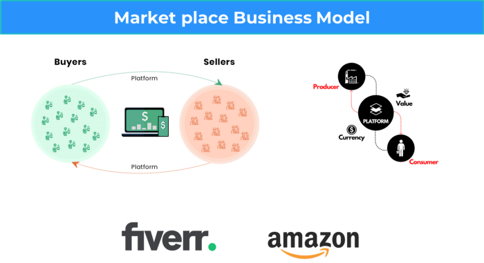
On Amazon's marketplace, a third-party vendor sells a product.
Freelancers on Fiverr offer specialized skills like graphic design.
Marketplace's business concept is explained.
4. Business plans using aggregates
In the aggregator business model, the service is branded.
Uber, Airbnb, and other examples
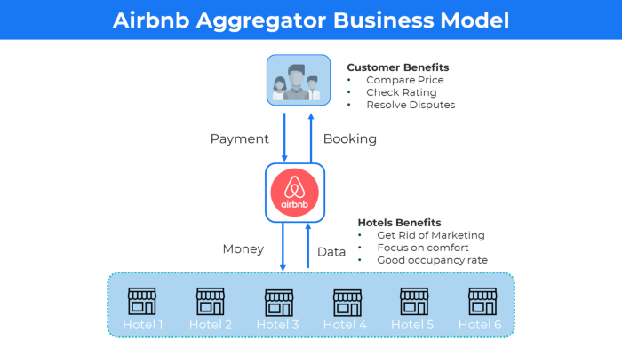
Marketplace and Aggregator business models differ.
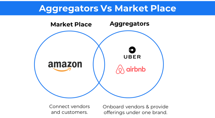
Amazon and Fiverr link merchants and customers and take a 10-20% revenue split.
Uber and Airbnb-style aggregator Join these businesses and provide their products.
5. The pay-as-you-go concept of business
This is a consumption-based pricing system. Cloud companies use it.
Example: Amazon Web Service and Google Cloud Platform (GCP) (AWS)
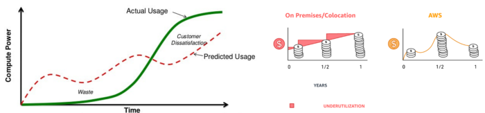
AWS, an Amazon subsidiary, offers over 200 pay-as-you-go cloud services.
“In short, the more you use the more you pay”
When it's difficult to divide clients into pricing levels, pay-as-you is employed.
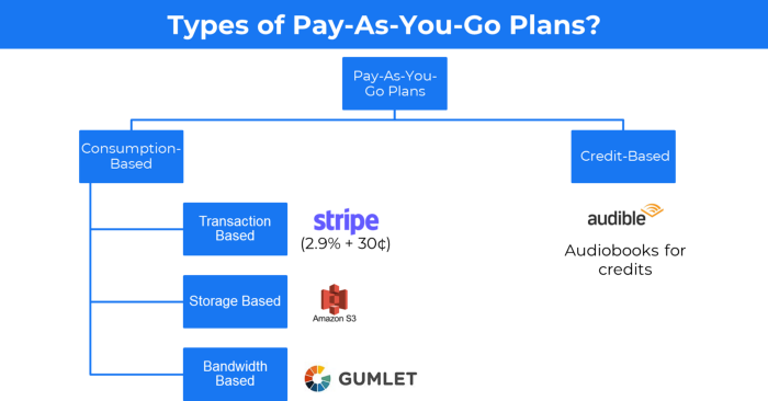
6. The business model known as fee-for-service (FFS)
FFS charges fixed and variable fees for each successful payment.
For instance, PayU, Paypal, and Stripe
Stripe charges 2.9% + 30 per payment.
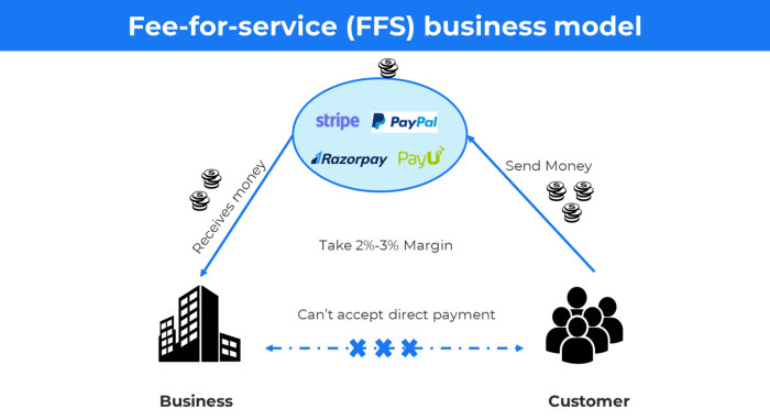
These firms offer a payment gateway to take consumer payments and deposit them to a business account.
Fintech business model
7. EdTech business strategy
In edtech, you generate money by selling material or teaching as a service.
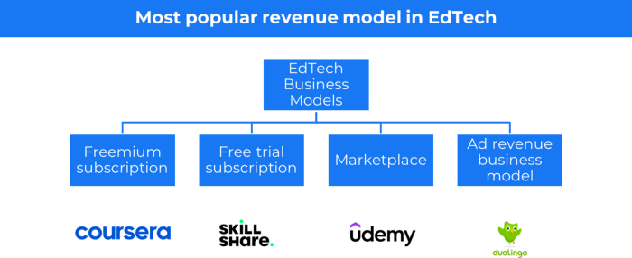
edtech business models
Freemium When course content is free but certification isn't, e.g. Coursera
FREE TRIAL SkillShare offers free trials followed by monthly or annual subscriptions.
Self-serving marketplace approach where you pick what to learn.
Ad-revenue model The company makes money by showing adverts to its huge user base.
Lock-in business strategy
Lock in prevents customers from switching to a competitor's brand or offering.
It uses switching costs or effort to transmit (soft lock-in), improved brand experience, or incentives.
Apple, SAP, and other examples
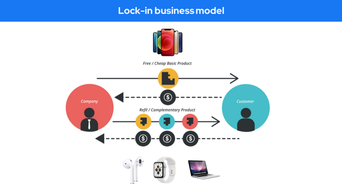
Apple offers an iPhone and then locks you in with extra hardware (Watch, Airpod) and platform services (Apple Store, Apple Music, cloud, etc.).
9. Business Model for API Licensing
APIs let third-party apps communicate with your service.
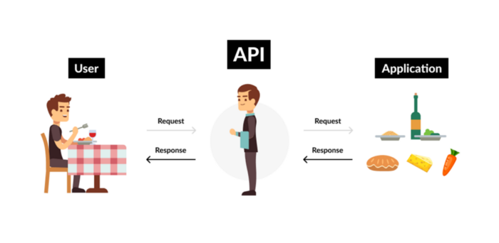
Uber and Airbnb use Google Maps APIs for app navigation.
Examples are Google Map APIs (Map), Sendgrid (Email), and Twilio (SMS).
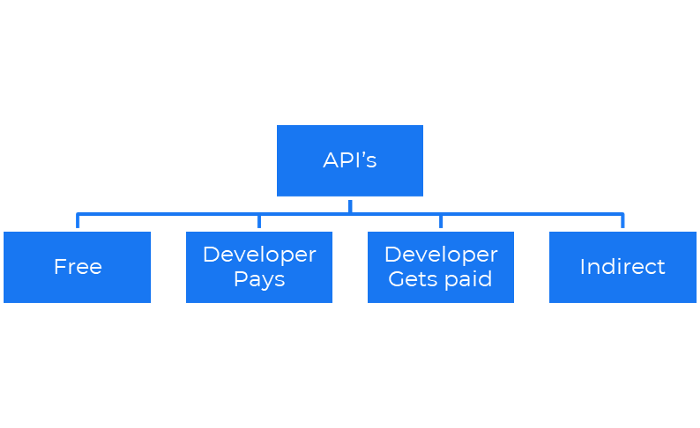
Business models for APIs
Free: The simplest API-driven business model that enables unrestricted API access for app developers. Google Translate and Facebook are two examples.
Developer Pays: Under this arrangement, service providers such as AWS, Twilio, Github, Stripe, and others must be paid by application developers.
The developer receives payment: These are the compensated content producers or developers who distribute the APIs utilizing their work. For example, Amazon affiliate programs
10. Open-source enterprise
Open-source software can be inspected, modified, and improved by anybody.
For instance, use Firefox, Java, or Android.

Google paid Mozilla $435,702 million to be their primary search engine in 2018.
Open-source software profits in six ways.
Paid assistance The Project Manager can charge for customization because he is quite knowledgeable about the codebase.
A full database solution is available as a Software as a Service (MongoDB Atlas), but there is a fee for the monitoring tool.
Open-core design R studio is a better GUI substitute for open-source applications.
sponsors of GitHub Sponsorships benefit the developers in full.
demands for paid features Earn Money By Developing Open Source Add-Ons for Current Products
Open-source business model
11. The business model for data
If the software or algorithm collects client data to improve or monetize the system.
Open AI GPT3 gets smarter with use.
Foursquare allows users to exchange check-in locations.
Later, they compiled large datasets to enable retailers like Starbucks launch new outlets.
12. Business Model Using Blockchain
Blockchain is a distributed ledger technology that allows firms to deploy smart contracts without a central authority.
Examples include Alchemy, Solana, and Ethereum.
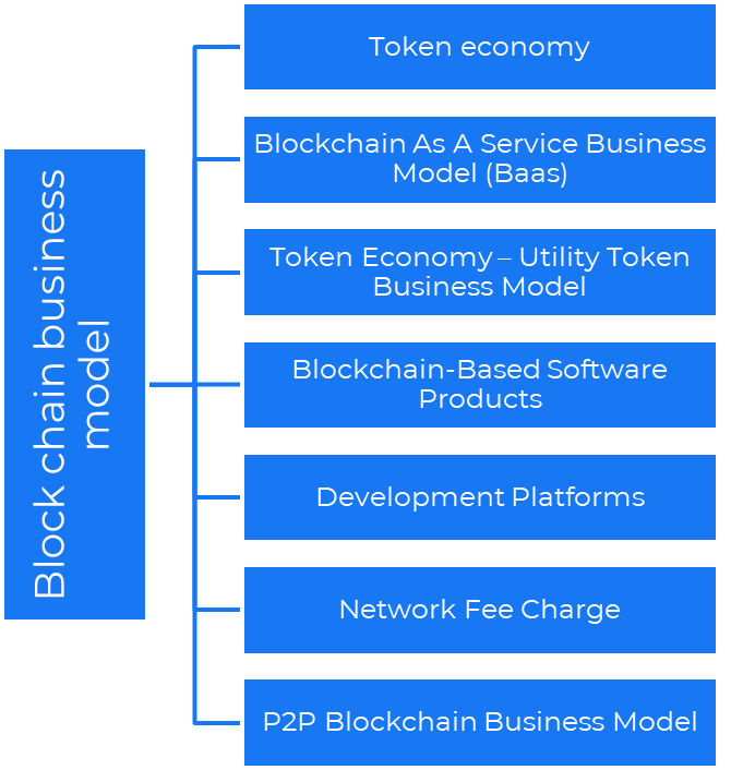
Business models using blockchain
Economy of tokens or utility When a business uses a token business model, it issues some kind of token as one of the ways to compensate token holders or miners. For instance, Solana and Ethereum
Bitcoin Cash P2P Business Model Peer-to-peer (P2P) blockchain technology permits direct communication between end users. as in IPFS
Enterprise Blockchain as a Service (Baas) BaaS focuses on offering ecosystem services similar to those offered by Amazon (AWS) and Microsoft (Azure) in the web 3 sector. Example: Ethereum Blockchain as a Service with Bitcoin (EBaaS).
Blockchain-Based Aggregators With AWS for blockchain, you can use that service by making an API call to your preferred blockchain. As an illustration, Alchemy offers nodes for many blockchains.
13. The free-enterprise model
In the freeterprise business model, free professional accounts are led into the funnel by the free product and later become B2B/enterprise accounts.
For instance, Slack and Zoom
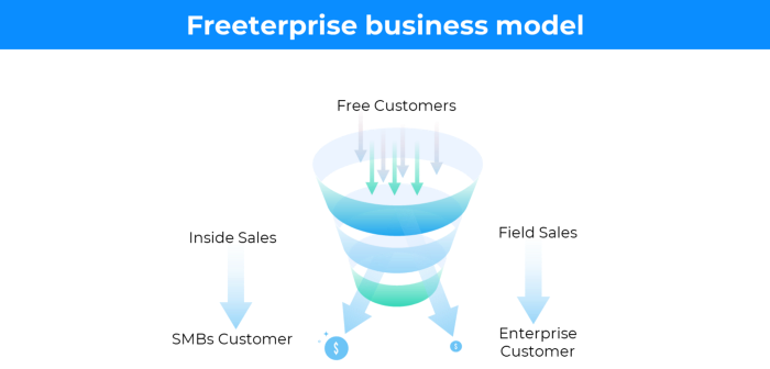
Freeterprise companies flourish through collaboration.
Start with a free professional account to build an enterprise.
14. Business plan for razor blades
It's employed in hardware where one piece is sold at a loss and profits are made through refills or add-ons.
Gillet razor & blades, coffee machine & beans, HP printer & cartridge, etc.
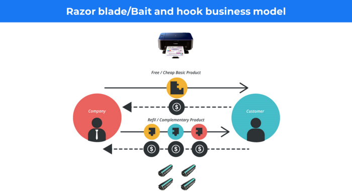
Sony sells the Playstation console at a loss but makes up for it by selling games and charging for online services.
Advantages of the Razor-Razorblade Method
lowers the risk a customer will try a product. enables buyers to test the goods and services without having to pay a high initial investment.
The product's ongoing revenue stream has the potential to generate sales that much outweigh the original investments.
Razor blade business model
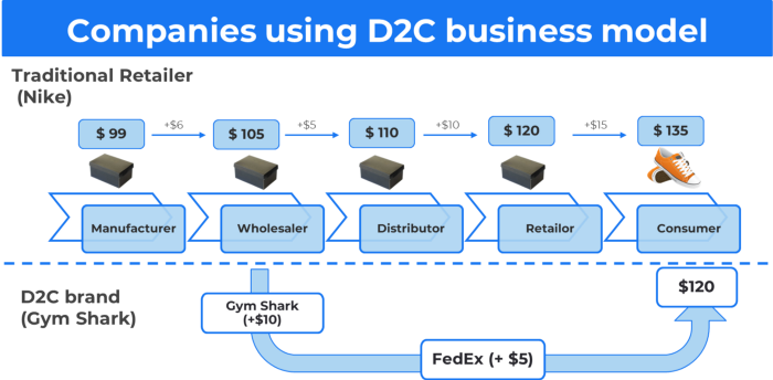
15. The business model of direct-to-consumer (D2C)
In D2C, the company sells directly to the end consumer through its website using a third-party logistic partner.
Examples include GymShark and Kylie Cosmetics.
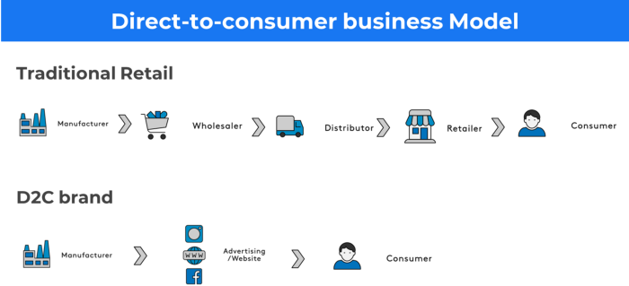
D2C brands can only expand via websites, marketplaces (Amazon, eBay), etc.
D2C benefits
Lower reliance on middlemen = greater profitability
You now have access to more precise demographic and geographic customer data.
Additional space for product testing
Increased customisation throughout your entire product line-Inventory Less
16. Business model: White Label vs. Private Label
Private label/White label products are made by a contract or third-party manufacturer.
Most amazon electronics are made in china and white-labeled.
Amazon supplements and electronics.
Contract manufacturers handle everything after brands select product quantities on design labels.
17. The franchise model
The franchisee uses the franchisor's trademark, branding, and business strategy (company).
For instance, KFC, Domino's, etc.
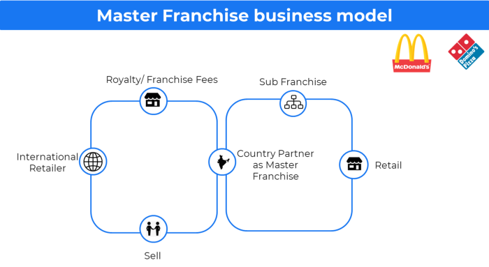
Subway, Domino, Burger King, etc. use this business strategy.
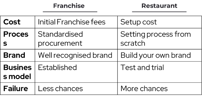
Many people pick a franchise because opening a restaurant is risky.
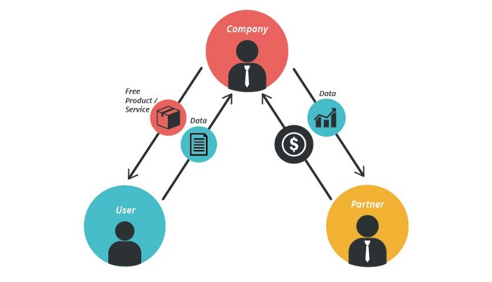
18. Ad-based business model
Social media and search engine giants exploit search and interest data to deliver adverts.
Google, Meta, TikTok, and Snapchat are some examples.
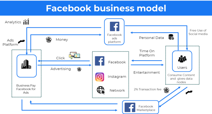
Users don't pay for the service or product given, e.g. Google users don't pay for searches.
In exchange, they collected data and hyper-personalized adverts to maximize revenue.
19. Business plan for octopuses
Each business unit functions separately but is connected to the main body.
Instance: Oyo
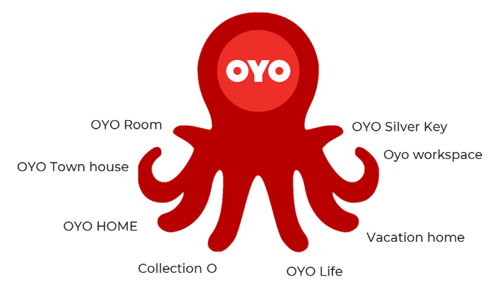
OYO is Asia's Airbnb, operating hotels, co-working, co-living, and vacation houses.
20, Transactional business model, number
Sales to customers produce revenue.
E-commerce sites and online purchases employ SSL.
Goli is an ex-GymShark.
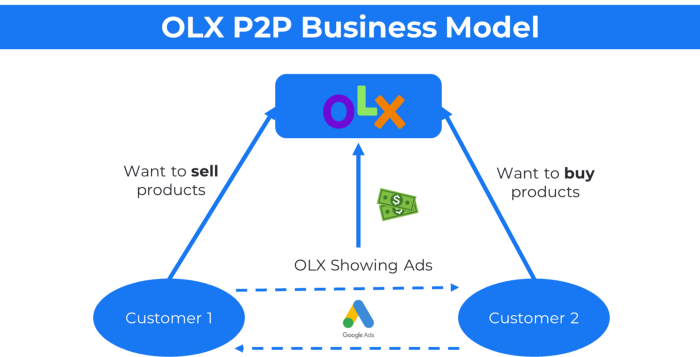
21. The peer-to-peer (P2P) business model
In P2P, two people buy and sell goods and services without a third party or platform.
Consider OLX.
22. P2P lending as a manner of operation
In P2P lending, one private individual (P2P Lender) lends/invests or borrows money from another (P2P Borrower).
Instance: Kabbage
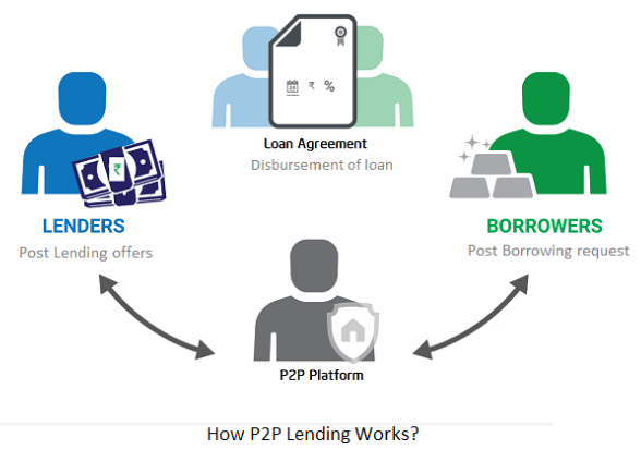
Social lending lets people lend and borrow money directly from each other without an intermediary financial institution.
23. A business model for brokers
Brokerages charge a commission or fee for their services.
Examples include eBay, Coinbase, and Robinhood.
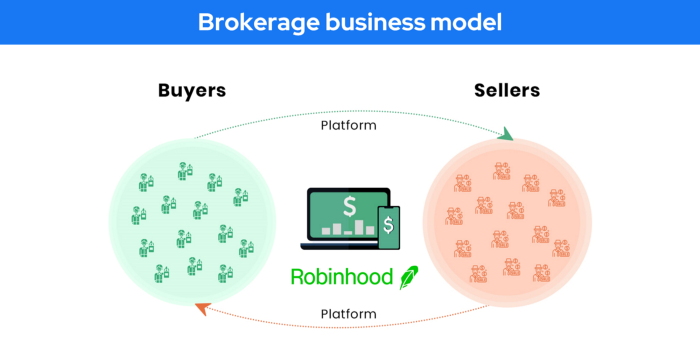
Brokerage businesses are common in Real estate, finance, and online and operate on this model.
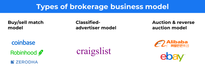
Buy/sell similar models Examples include financial brokers, insurance brokers, and others who match purchase and sell transactions and charge a commission.
These brokers charge an advertiser a fee based on the date, place, size, or type of an advertisement. This is known as the classified-advertiser model. For instance, Craiglist
24. Drop shipping as an industry
Dropshipping allows stores to sell things without holding physical inventories.
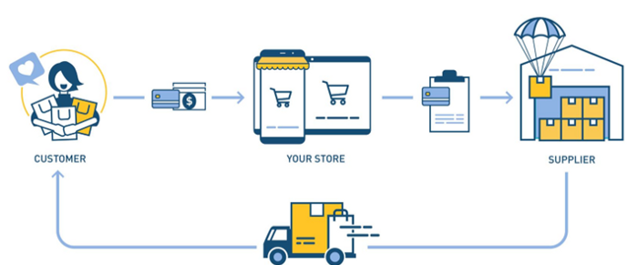
When a customer orders, use a third-party supplier and logistic partners.
Retailer product portfolio and customer experience Fulfiller The consumer places the order.
Dropshipping advantages
Less money is needed (Low overhead-No Inventory or warehousing)
Simple to start (costs under $100)
flexible work environment
New product testing is simpler
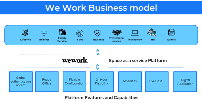
25. Business Model for Space as a Service
It's centered on a shared economy that lets millennials live or work in communal areas without ownership or lease.
Consider WeWork and Airbnb.
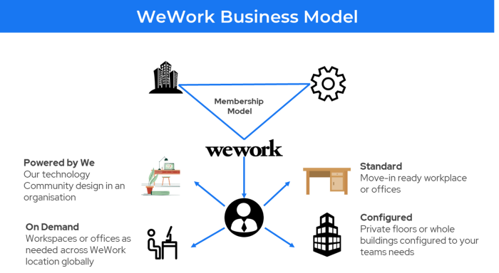
WeWork helps businesses with real estate, legal compliance, maintenance, and repair.
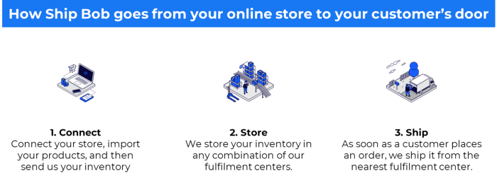
26. The business model for third-party logistics (3PL)
In 3PL, a business outsources product delivery, warehousing, and fulfillment to an external logistics company.
Examples include Ship Bob, Amazon Fulfillment, and more.

3PL partners warehouse, fulfill, and return inbound and outbound items for a charge.
Inbound logistics involves bringing products from suppliers to your warehouse.
Outbound logistics refers to a company's production line, warehouse, and customer.
27. The last-mile delivery paradigm as a commercial strategy
Last-mile delivery is the collection of supply chain actions that reach the end client.
Examples include Rappi, Gojek, and Postmates.
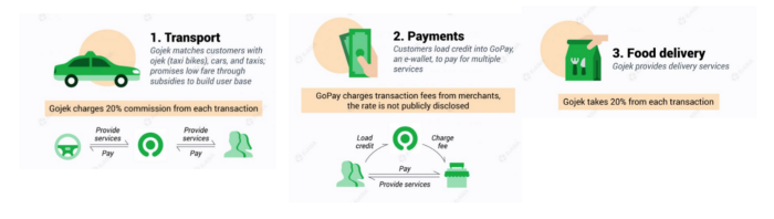
Last-mile is tied to on-demand and has a nighttime peak.
28. The use of affiliate marketing
Affiliate marketing involves promoting other companies' products and charging commissions.
Examples include Hubspot, Amazon, and Skillshare.
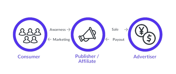
Your favorite youtube channel probably uses these short amazon links to get 5% of sales.
Affiliate marketing's benefits
In exchange for a success fee or commission, it enables numerous independent marketers to promote on its behalf.
Ensure system transparency by giving the influencers a specific tracking link and an online dashboard to view their profits.
Learn about the newest bargains and have access to promotional materials.
29. The business model for virtual goods
This is an in-app purchase for an intangible product.
Examples include PubG, Roblox, Candy Crush, etc.
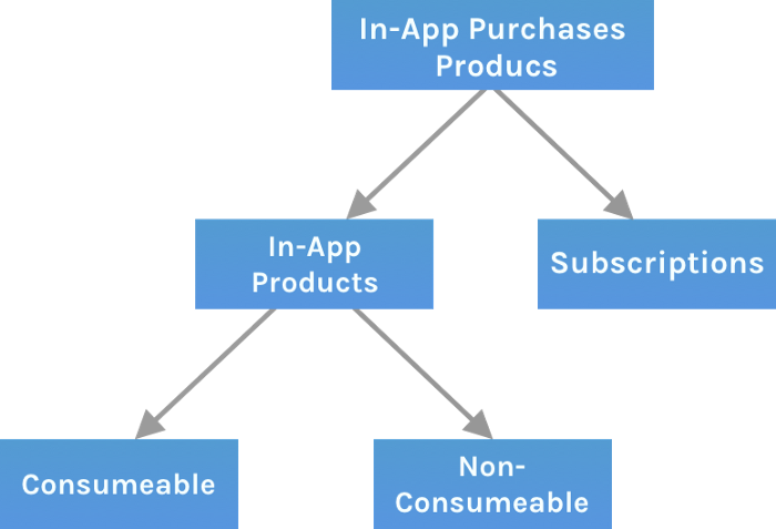
Consumables are like gaming cash that runs out. Non-consumable products provide a permanent advantage without repeated purchases.
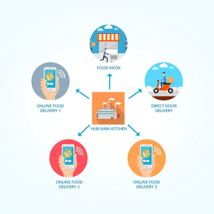
30. Business Models for Cloud Kitchens
Ghost, Dark, Black Box, etc.
Delivery-only restaurant.
These restaurants don't provide dine-in, only delivery.
For instance, NextBite and Faasos
31. Crowdsourcing as a Business Model
Crowdsourcing = Using the crowd as a platform's source.
In crowdsourcing, you get support from people around the world without hiring them.
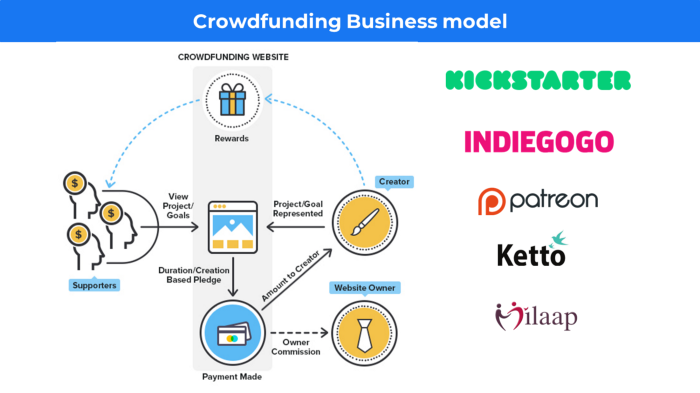
Crowdsourcing sites
Open-Source Software gives access to the software's source code so that developers can edit or enhance it. Examples include Firefox browsers and Linux operating systems.
Crowdfunding The oculus headgear would be an example of crowdfunding in essence, with no expectations.

Sofien Kaabar, CFA
3 years ago
How to Make a Trading Heatmap
Python Heatmap Technical Indicator

Heatmaps provide an instant overview. They can be used with correlations or to predict reactions or confirm the trend in trading. This article covers RSI heatmap creation.
The Market System
Market regime:
Bullish trend: The market tends to make higher highs, which indicates that the overall trend is upward.
Sideways: The market tends to fluctuate while staying within predetermined zones.
Bearish trend: The market has the propensity to make lower lows, indicating that the overall trend is downward.
Most tools detect the trend, but we cannot predict the next state. The best way to solve this problem is to assume the current state will continue and trade any reactions, preferably in the trend.
If the EURUSD is above its moving average and making higher highs, a trend-following strategy would be to wait for dips before buying and assuming the bullish trend will continue.
Indicator of Relative Strength
J. Welles Wilder Jr. introduced the RSI, a popular and versatile technical indicator. Used as a contrarian indicator to exploit extreme reactions. Calculating the default RSI usually involves these steps:
Determine the difference between the closing prices from the prior ones.
Distinguish between the positive and negative net changes.
Create a smoothed moving average for both the absolute values of the positive net changes and the negative net changes.
Take the difference between the smoothed positive and negative changes. The Relative Strength RS will be the name we use to describe this calculation.
To obtain the RSI, use the normalization formula shown below for each time step.
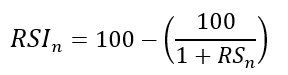

The 13-period RSI and black GBPUSD hourly values are shown above. RSI bounces near 25 and pauses around 75. Python requires a four-column OHLC array for RSI coding.
import numpy as np
def add_column(data, times):

    for i in range(1, times + 1):

        new = np.zeros((len(data), 1), dtype = float)

        data = np.append(data, new, axis = 1)
    return data
def delete_column(data, index, times):

    for i in range(1, times + 1):

        data = np.delete(data, index, axis = 1)
    return data
def delete_row(data, number):

    data = data[number:, ]

    return data
def ma(data, lookback, close, position):

    data = add_column(data, 1)

    for i in range(len(data)):

            try:

                data[i, position] = (data[i - lookback + 1:i + 1, close].mean())

            except IndexError:

                pass

    data = delete_row(data, lookback)

    return data
def smoothed_ma(data, alpha, lookback, close, position):

    lookback = (2 * lookback) - 1

    alpha = alpha / (lookback + 1.0)

    beta  = 1 - alpha

    data = ma(data, lookback, close, position)
    data[lookback + 1, position] = (data[lookback + 1, close] * alpha) + (data[lookback, position] * beta)
    for i in range(lookback + 2, len(data)):

            try:

                data[i, position] = (data[i, close] * alpha) + (data[i - 1, position] * beta)

            except IndexError:

                pass

    return data
def rsi(data, lookback, close, position):

    data = add_column(data, 5)

    for i in range(len(data)):

        data[i, position] = data[i, close] - data[i - 1, close]

    for i in range(len(data)):

        if data[i, position] > 0:

            data[i, position + 1] = data[i, position]

        elif data[i, position] < 0:

            data[i, position + 2] = abs(data[i, position])

    data = smoothed_ma(data, 2, lookback, position + 1, position + 3)
    data = smoothed_ma(data, 2, lookback, position + 2, position + 4)
    data[:, position + 5] = data[:, position + 3] / data[:, position + 4]

    data[:, position + 6] = (100 - (100 / (1 + data[:, position + 5])))
    data = delete_column(data, position, 6)
    data = delete_row(data, lookback)
    return data
Make sure to focus on the concepts and not the code. You can find the codes of most of my strategies in my books. The most important thing is to comprehend the techniques and strategies.
My weekly market sentiment report uses complex and simple models to understand the current positioning and predict the future direction of several major markets. Check out the report here:
Using the Heatmap to Find the Trend
RSI trend detection is easy but useless. Bullish and bearish regimes are in effect when the RSI is above or below 50, respectively. Tracing a vertical colored line creates the conditions below. How:
When the RSI is higher than 50, a green vertical line is drawn.
When the RSI is lower than 50, a red vertical line is drawn.
Zooming out yields a basic heatmap, as shown below.

Plot code:
def indicator_plot(data, second_panel, window = 250):
    fig, ax = plt.subplots(2, figsize = (10, 5))
    sample = data[-window:, ]
    for i in range(len(sample)):
        ax[0].vlines(x = i, ymin = sample[i, 2], ymax = sample[i, 1], color = 'black', linewidth = 1)
        if sample[i, 3] > sample[i, 0]:
            ax[0].vlines(x = i, ymin = sample[i, 0], ymax = sample[i, 3], color = 'black', linewidth = 1.5)
        if sample[i, 3] < sample[i, 0]:
            ax[0].vlines(x = i, ymin = sample[i, 3], ymax = sample[i, 0], color = 'black', linewidth = 1.5)
        if sample[i, 3] == sample[i, 0]:
            ax[0].vlines(x = i, ymin = sample[i, 3], ymax = sample[i, 0], color = 'black', linewidth = 1.5)
    ax[0].grid()
    for i in range(len(sample)):
        if sample[i, second_panel] > 50:
            ax[1].vlines(x = i, ymin = 0, ymax = 100, color = 'green', linewidth = 1.5)
        if sample[i, second_panel] < 50:
            ax[1].vlines(x = i, ymin = 0, ymax = 100, color = 'red', linewidth = 1.5)
    ax[1].grid()
indicator_plot(my_data, 4, window = 500)
Call RSI on your OHLC array's fifth column. 4. Adjusting lookback parameters reduces lag and false signals. Other indicators and conditions are possible.
Another suggestion is to develop an RSI Heatmap for Extreme Conditions.
Contrarian indicator RSI. The following rules apply:
Whenever the RSI is approaching the upper values, the color approaches red.
The color tends toward green whenever the RSI is getting close to the lower values.
Zooming out yields a basic heatmap, as shown below.

Plot code:
import matplotlib.pyplot as plt
def indicator_plot(data, second_panel, window = 250):
    fig, ax = plt.subplots(2, figsize = (10, 5))
    sample = data[-window:, ]
    for i in range(len(sample)):
        ax[0].vlines(x = i, ymin = sample[i, 2], ymax = sample[i, 1], color = 'black', linewidth = 1)
        if sample[i, 3] > sample[i, 0]:
            ax[0].vlines(x = i, ymin = sample[i, 0], ymax = sample[i, 3], color = 'black', linewidth = 1.5)
        if sample[i, 3] < sample[i, 0]:
            ax[0].vlines(x = i, ymin = sample[i, 3], ymax = sample[i, 0], color = 'black', linewidth = 1.5)
        if sample[i, 3] == sample[i, 0]:
            ax[0].vlines(x = i, ymin = sample[i, 3], ymax = sample[i, 0], color = 'black', linewidth = 1.5)
    ax[0].grid()
    for i in range(len(sample)):
        if sample[i, second_panel] > 90:
            ax[1].vlines(x = i, ymin = 0, ymax = 100, color = 'red', linewidth = 1.5)
        if sample[i, second_panel] > 80 and sample[i, second_panel] < 90:
            ax[1].vlines(x = i, ymin = 0, ymax = 100, color = 'darkred', linewidth = 1.5)
        if sample[i, second_panel] > 70 and sample[i, second_panel] < 80:
            ax[1].vlines(x = i, ymin = 0, ymax = 100, color = 'maroon', linewidth = 1.5)
        if sample[i, second_panel] > 60 and sample[i, second_panel] < 70:
            ax[1].vlines(x = i, ymin = 0, ymax = 100, color = 'firebrick', linewidth = 1.5)
        if sample[i, second_panel] > 50 and sample[i, second_panel] < 60:
            ax[1].vlines(x = i, ymin = 0, ymax = 100, color = 'grey', linewidth = 1.5)
        if sample[i, second_panel] > 40 and sample[i, second_panel] < 50:
            ax[1].vlines(x = i, ymin = 0, ymax = 100, color = 'grey', linewidth = 1.5)
        if sample[i, second_panel] > 30 and sample[i, second_panel] < 40:
            ax[1].vlines(x = i, ymin = 0, ymax = 100, color = 'lightgreen', linewidth = 1.5)
        if sample[i, second_panel] > 20 and sample[i, second_panel] < 30:
            ax[1].vlines(x = i, ymin = 0, ymax = 100, color = 'limegreen', linewidth = 1.5)
        if sample[i, second_panel] > 10 and sample[i, second_panel] < 20:
            ax[1].vlines(x = i, ymin = 0, ymax = 100, color = 'seagreen', linewidth = 1.5)
        if sample[i, second_panel] > 0 and sample[i, second_panel] < 10:
            ax[1].vlines(x = i, ymin = 0, ymax = 100, color = 'green', linewidth = 1.5)
    ax[1].grid()
indicator_plot(my_data, 4, window = 500)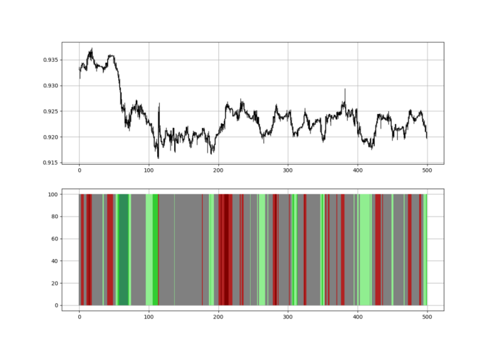
Dark green and red areas indicate imminent bullish and bearish reactions, respectively. RSI around 50 is grey.
Summary
To conclude, my goal is to contribute to objective technical analysis, which promotes more transparent methods and strategies that must be back-tested before implementation.
Technical analysis will lose its reputation as subjective and unscientific.
When you find a trading strategy or technique, follow these steps:
Put emotions aside and adopt a critical mindset.
Test it in the past under conditions and simulations taken from real life.
Try optimizing it and performing a forward test if you find any potential.
Transaction costs and any slippage simulation should always be included in your tests.
Risk management and position sizing should always be considered in your tests.
After checking the above, monitor the strategy because market dynamics may change and make it unprofitable.