


More on Entrepreneurship/Creators
Maddie Wang
3 years ago
Easiest and fastest way to test your startup idea!
Here's the fastest way to validate company concepts.
I squandered a year after dropping out of Stanford designing a product nobody wanted.
But today, I’m at 100k!
Differences:
I was designing a consumer product when I dropped out.
I coded MVP, got 1k users, and got YC interview.
Nice, huh?
WRONG!
Still coding and getting users 12 months later
WOULD PEOPLE PAY FOR IT? was the riskiest assumption I hadn't tested.
When asked why I didn't verify payment, I said,
Not-ready products. Now, nobody cares. The website needs work. Include this. Increase usage…
I feared people would say no.
After 1 year of pushing it off, my team told me they were really worried about the Business Model. Then I asked my audience if they'd buy my product.
So?
No, overwhelmingly.
I felt like I wasted a year building a product no one would buy.
Founders Cafe was the opposite.
Before building anything, I requested payment.
40 founders were interviewed.
Then we emailed Stanford, YC, and other top founders, asking them to join our community.
BOOM! 10/12 paid!
Without building anything, in 1 day I validated my startup's riskiest assumption. NOT 1 year.
Asking people to pay is one of the scariest things.
I understand.
I asked Stanford queer women to pay before joining my gay sorority.
I was afraid I'd turn them off or no one would pay.
Gay women, like those founders, were in such excruciating pain that they were willing to pay me upfront to help.
You can ask for payment (before you build) to see if people have the burning pain. Then they'll pay!
Examples from Founders Cafe members:
😮 Using a fake landing page, a college dropout tested a product. Paying! He built it and made $3m!
😮 YC solo founder faked a Powerpoint demo. 5 Enterprise paid LOIs. $1.5m raised, built, and in YC!
😮 A Harvard founder can convert Figma to React. 1 day, 10 customers. Built a tool to automate Figma -> React after manually fulfilling requests. 1m+
Bad example:
😭 Stanford Dropout Spends 1 Year Building Product Without Payment Validation
Some people build for a year and then get paying customers.
What I'm sharing is my experience and what Founders Cafe members have told me about validating startup ideas.
Don't waste a year like I did.
After my first startup failed, I planned to re-enroll at Stanford/work at Facebook.
After people paid, I quit for good.
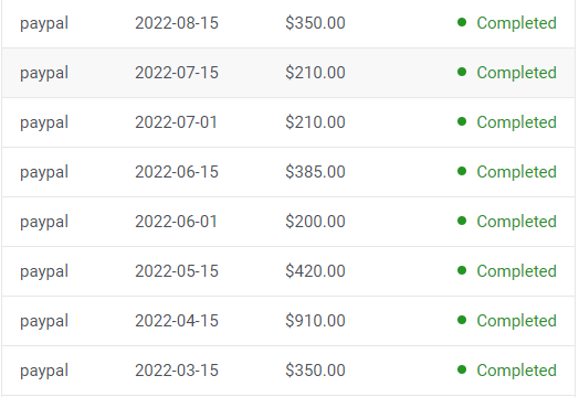
I've hit $100k!
Hope this inspires you to request upfront payment! It'll change your life

Hasan AboulHasan
3 years ago
High attachment products can help you earn money automatically.
Affiliate marketing is a popular online moneymaker. You promote others' products and get commissions. Affiliate marketing requires constant product promotion.
Affiliate marketing can be profitable even without much promotion. Yes, this is Autopilot Money.
How to Pick an Affiliate Program to Generate Income Autonomously
Autopilot moneymaking requires a recurring affiliate marketing program.
Finding the best product and testing it takes a lot of time and effort.
Here are three ways to choose the best service or product to promote:
Find a good attachment-rate product or service.
When choosing a product, ask if you can easily switch to another service. Attachment rate is how much people like a product.
Higher attachment rates mean better Autopilot products.
Consider promoting GetResponse. It's a 33% recurring commission email marketing tool. This means you get 33% of the customer's plan as long as he pays.
GetResponse has a high attachment rate because it's hard to leave and start over with another tool.
2. Pick a good or service with a lot of affiliate assets.
Check if a program has affiliate assets or creatives before joining.
Images and banners to promote the product in your business.
They save time; I look for promotional creatives. Creatives or affiliate assets are website banners or images. This reduces design time.
3. Select a service or item that consumers already adore.
New products are hard to sell. Choosing a trusted company's popular product or service is helpful.
As a beginner, let people buy a product they already love.
Online entrepreneurs and digital marketers love Systeme.io. It offers tools for creating pages, email marketing, funnels, and more. This product guarantees a high ROI.
Make the product known!
Affiliate marketers struggle to get traffic. Using affiliate marketing to make money is easier than you think if you have a solid marketing strategy.
Your plan should include:
1- Publish affiliate-related blog posts and SEO-optimize them
2- Sending new visitors product-related emails
3- Create a product resource page.
4-Review products
5-Make YouTube videos with links in the description.
6- Answering FAQs about your products and services on your blog and Quora.
7- Create an eCourse on how to use this product.
8- Adding Affiliate Banners to Your Website.
With these tips, you can promote your products and make money on autopilot.

Esteban
3 years ago
The Berkus Startup Valuation Method: What Is It?
What Is That?
Berkus is a pre-revenue valuation method based exclusively on qualitative criteria, like Scorecard.
Few firms match their financial estimates, especially in the early stages, so valuation methodologies like the Berkus method are a good way to establish a valuation when the economic measures are not reliable.
How does it work?
This technique evaluates five key success factors.
Fundamental principle
Technology
Execution
Strategic alliances in its primary market
Production, followed by sales
The Berkus technique values the business idea and four success factors. As seen in the matrix below, each of these dimensions poses a danger to the startup's success.
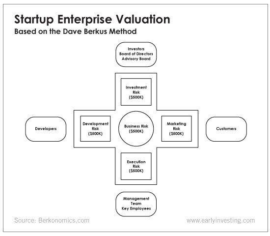
It assigns $0-$500,000 to each of these beginning regions. This approach enables a maximum $2.5M pre-money valuation.
This approach relies significantly on geography and uses the US as a baseline, as it differs in every country in Europe.
A set of standards for analyzing each dimension individually
Fundamental principle (or strength of the idea)
Ideas are worthless; execution matters. Most of us can relate to seeing a new business open in our area or a startup get funded and thinking, "I had this concept years ago!" Someone did it.
The concept remains. To assess the idea's viability, we must consider several criteria.
The concept's exclusivity It is necessary to protect a product or service's concept using patents and copyrights. Additionally, it must be capable of generating large profits.
Planned growth and growth that goes in a specific direction have a lot of potential, therefore incorporating them into a business is really advantageous.
The ability of a concept to grow A venture's ability to generate scalable revenue is a key factor in its emergence and continuation. A startup needs a scalable idea in order to compete successfully in the market.
The attraction of a business idea to a broad spectrum of people is significantly influenced by the current socio-political climate. Thus, the requirement for the assumption of conformity.
Concept Validation Ideas must go through rigorous testing with a variety of audiences in order to lower risk during the implementation phase.
Technology (Prototype)
This aspect reduces startup's technological risk. How good is the startup prototype when facing cyber threats, GDPR compliance (in Europe), tech stack replication difficulty, etc.?
Execution
Check the management team's efficacy. A potential angel investor must verify the founders' experience and track record with previous ventures. Good leadership is needed to chart a ship's course.
Strategic alliances in its primary market
Existing and new relationships will play a vital role in the development of both B2B and B2C startups. What are the startup's synergies? potential ones?
Production, followed by sales (product rollout)
Startup success depends on its manufacturing and product rollout. It depends on the overall addressable market, the startup's ability to market and sell their product, and their capacity to provide consistent, high-quality support.
Example
We're now founders of EyeCaramba, a machine vision-assisted streaming platform. My imagination always goes to poor puns when naming a startup.
Since we're first-time founders and the Berkus technique depends exclusively on qualitative methods and the evaluator's skill, we ask our angel-investor acquaintance for a pre-money appraisal of EyeCaramba.
Our friend offers us the following table:
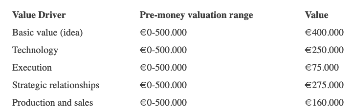
Because we're first-time founders, our pal lowered our Execution score. He knows the idea's value and that the gaming industry is red-hot, with worse startup ideas getting funded, therefore he gave the Basic value the highest value (idea).
EyeCaramba's pre-money valuation is $400,000 + $250,000 + $75,000 + $275,000 + $164,000 (1.16M). Good.
References
https://medium.com/humble-ventures/how-angel-investors-value-pre-revenue-startups-part-iii-8271405f0774#:~:text=pre%2Drevenue%20startups.-,Berkus%20Method,potential%20of%20the%20idea%20itself.%E2%80%9D
https://eqvista.com/berkus-valuation-method-for-startups/
https://www.venionaire.com/early-stage-startup-valuation-part-2-the-berkus-method/
You might also like

Tora Northman
3 years ago
Pixelmon NFTs are so bad, they are almost good!
Bored Apes prices continue to rise, HAPEBEAST launches, Invisible Friends hype continues to grow. Sadly, not all projects are as successful.
Of course, there are many factors to consider when buying an NFT. Is the project a scam? Will the reveal derail the project? Possibly, but when Pixelmon first teased its launch, it generated a lot of buzz.
With a primary sale mint price of 3 ETH ($8,100 USD), it started as an expensive project, with plenty of fans willing to invest in what was sold as a game. After it was revealed, it fell rapidly.
Why? It was overpromised and under delivered.
According to the project's creator[^1], the funds generated will be used to develop the artwork. "The Pixelmon reveal was wrong. This is what our Pixelmon look like in-game. "Despite the fud, I will not go anywhere," he wrote on Twitter. The goal remains. The funds will still be used to build our game. I will finish this project."
The project raised $70 million USD, but the NFTs buyers received were not the project's original teasers. Some call it "the worst NFT project ever," while others call it a complete scam.
But there's hope for some buyers. Kevin emerged from the ashes as the project was roasted over the fire.
A Minecraft character meets Salad Fingers - that's Kevin. He's a frog-like creature whose reveal was such a terrible NFT that it became part of history – and a meme.
If you're laughing at people paying $8K for a silly pixelated image, you might need to take it back. Precisely because of this, lucky holders who minted Kevin have been able to sell the now-memed NFT for over 8 ETH (around $24,000 USD), with some currently listed for 100 ETH.
Of course, Twitter has been awash in memes mocking those who invested in the project, because what else can you do when so many people lose money?
It's still unclear if the NFT project is a scam, but the team behind it was hired on Upwork. There's still hope for redemption, but Kevin's rise to fame appears to be the only positive outcome so far.
[^1] This is not the first time the creator (A 20-yo New Zealanders) has sought money via an online platform and had people claiming he under-delivered. He raised $74,000 on Kickstarter for a card game called Psycho Chicken. There are hundreds of comments on the Kickstarter project saying they haven't received the product and pleading for a refund or an update.

Scott Galloway
3 years ago
Don't underestimate the foolish
ZERO GRACE/ZERO MALICE
Big companies and wealthy people make stupid mistakes too.
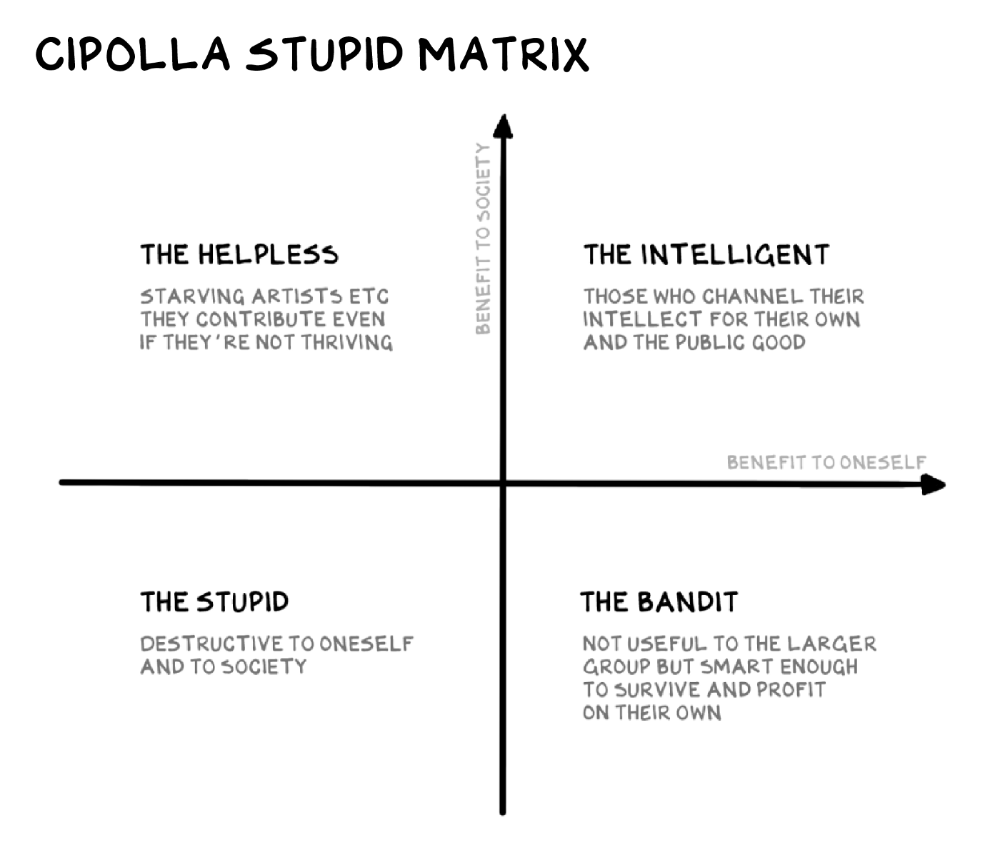
Your ancestors kept snakes and drank bad water. You (probably) don't because you've learnt from their failures via instinct+, the ultimate life-lessons streaming network in your head. Instincts foretell the future. If you approach a lion, it'll eat you. Our society's nuanced/complex decisions have surpassed instinct. Human growth depends on how we handle these issues. 80% of people believe they are above-average drivers, yet few believe they make many incorrect mistakes that make them risky. Stupidity hurts others like death. Basic Laws of Human Stupidity by Carlo Cipollas:
Everyone underestimates the prevalence of idiots in our society.
Any other trait a person may have has no bearing on how likely they are to be stupid.
A dumb individual is one who harms someone without benefiting themselves and may even lose money in the process.
Non-dumb people frequently underestimate how destructively powerful stupid people can be.
The most dangerous kind of person is a moron.
Professor Cippola defines stupid as bad for you and others. We underestimate the corporate world's and seemingly successful people's ability to make bad judgments that harm themselves and others. Success is an intoxication that makes you risk-aggressive and blurs your peripheral vision.
Stupid companies and decisions:
Big Dumber
Big-company bad ideas have more bulk and inertia. The world's most valuable company recently showed its board a VR headset. Jony Ive couldn't destroy Apple's terrible idea in 2015. Mr. Ive said that VR cut users off from the outer world, made them seem outdated, and lacked practical uses. Ives' design team doubted users would wear headsets for lengthy periods.
VR has cost tens of billions of dollars over a decade to prove nobody wants it. The next great SaaS startup will likely come from Florence, not Redmond or San Jose.
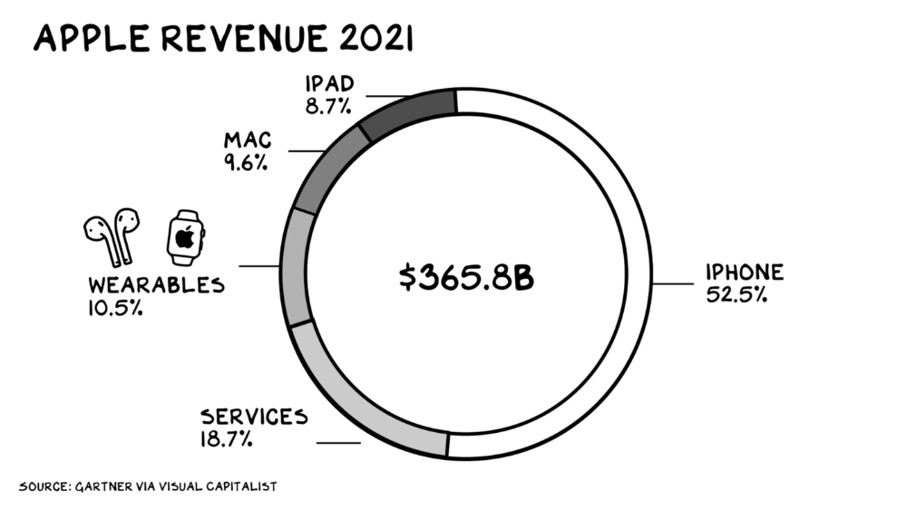
Apple Watch and Airpods have made the Cupertino company the world's largest jewelry maker. 10.5% of Apple's income, or $38 billion, comes from wearables in 2021. (seven times the revenue of Tiffany & Co.). Jewelry makes you more appealing and useful. Airpods and Apple Watch do both.
Headsets make you less beautiful and useful and promote isolation, loneliness, and unhappiness among American teenagers. My sons pretend they can't hear or see me when on their phones. VR headsets lack charisma.
Coinbase disclosed a plan to generate division and tension within its workplace weeks after Apple was pitched $2,000 smokes. The crypto-trading platform is piloting a program that rates staff after every interaction. If a coworker says anything you don't like, you should tell them how to improve. Everyone gets a 110-point scorecard. Coworkers should evaluate a person's rating while deciding whether to listen to them. It's ridiculous.
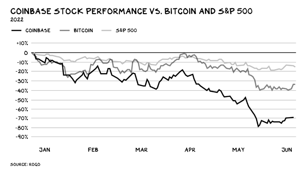
Organizations leverage our superpower of cooperation. This encourages non-cooperation, period. Bridgewater's founder Ray Dalio designed the approach to promote extreme transparency. Dalio has 223 billion reasons his managerial style works. There's reason to suppose only a small group of people, largely traders, will endure a granular scorecard. Bridgewater has 20% first-year turnover. Employees cry in bathrooms, and sex scandals are settled by ignoring individuals with poor believability levels. Coinbase might take solace that the stock is 80% below its initial offering price.
Poor Stupid
Fools' ledgers are valuable. More valuable are lists of foolish rich individuals.
Robinhood built a $8 billion corporation on financial ignorance. The firm's median account value is $240, and its stock has dropped 75% since last summer. Investors, customers, and society lose. Stupid. Luna published a comparable list on the blockchain, grew to $41 billion in market cap, then plummeted.
A podcast presenter is recruiting dentists and small-business owners to invest in Elon Musk's Twitter takeover. Investors pay a 7% fee and 10% of the upside for the chance to buy Twitter at a 35% premium to the current price. The proposal legitimizes CNBC's Trade Like Chuck advertising (Chuck made $4,600 into $460,000 in two years). This is stupid because it adds to the Twitter deal's desperation. Mr. Musk made an impression when he urged his lawyers to develop a legal rip-cord (There are bots on the platform!) to abandon the share purchase arrangement (for less than they are being marketed by the podcaster). Rolls-Royce may pay for this list of the dumb affluent because it includes potential Cullinan buyers.
Worst company? Flowcarbon, founded by WeWork founder Adam Neumann, operates at the convergence of carbon and crypto to democratize access to offsets and safeguard the earth's natural carbon sinks. Can I get an ayahuasca Big Gulp?
Neumann raised $70 million with their yogababble drink. More than half of the consideration came from selling GNT. Goddess Nature Token. I hope the company gets an S-1. Or I'll start a decentralized AI Meta Renewable NFTs company. My Community Based Ebitda coin will fund the company. Possible.
Stupidity inside oneself
This weekend, I was in NYC with my boys. My 14-year-old disappeared. He's realized I'm not cool and is mad I let the charade continue. When out with his dad, he likes to stroll home alone and depart before me. Friends told me hell would return, but I was surprised by how fast the eye roll came.
Not so with my 11-year-old. We went to The Edge, a Hudson Yards observation platform where you can see the city from 100 storeys up for $38. This is hell's seventh ring. Leaning into your boys' interests is key to engaging them (dad tip). Neither loves Crossfit, WW2 history, or antitrust law.
We take selfies on the Thrilling Glass Floor he spots. Dad, there's a bar! Coke? I nod, he rushes to the bar, stops, runs back for money, and sprints back. Sitting on stone seats, drinking Atlanta Champagne, he turns at me and asks, Isn't this amazing? I'll never reach paradise.
Later that night, the lads are asleep and I've had two Zacapas and Cokes. I SMS some friends about my day and how I feel about sons/fatherhood/etc. How I did. They responded and approached. The next morning, I'm sober, have distance from my son, and feel ashamed by my texts. Less likely to impulsively share my emotions with others. Stupid again.
Jumanne Rajabu Mtambalike
3 years ago
10 Years of Trying to Manage Time and Improve My Productivity.
I've spent the last 10 years of my career mastering time management. I've tried different approaches and followed multiple people and sources. My knowledge is summarized.
Great people, including entrepreneurs, master time management. I learned time management in college. I was studying Computer Science and Finance and leading Tanzanian students in Bangalore, India. I had 24 hours per day to do this and enjoy campus. I graduated and received several awards. I've learned to maximize my time. These tips and tools help me finish quickly.
Eisenhower-Box
I don't remember when I read the article. James Clear, one of my favorite bloggers, introduced me to the Eisenhower Box, which I've used for years. Eliminate waste to master time management. By grouping your activities by importance and urgency, the tool helps you prioritize what matters and drop what doesn't. If it's urgent, do it. Delegate if it's urgent but not necessary. If it's important but not urgent, reschedule it; otherwise, drop it. I integrated the tool with Trello to manage my daily tasks. Since 2007, I've done this.
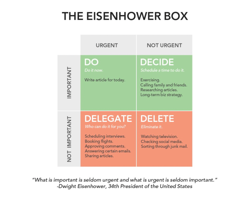
James Clear's article mentions Eisenhower Box.
Essentialism rules
Greg McKeown's book Essentialism introduced me to disciplined pursuit of less. I once wrote about this. I wasn't sure what my career's real opportunities and distractions were. A non-essentialist thinks everything is essential; you want to be everything to everyone, and your life lacks satisfaction. Poor time management starts it all. Reading and applying this book will change your life.
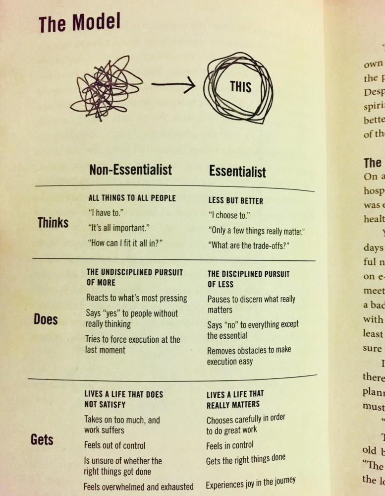
Essential vs non-essential
Life Calendar
Most of us make corporate calendars. Peter Njonjo, founder of Twiga Foods, said he manages time by putting life activities in his core calendars. It includes family retreats, weddings, and other events. He joked that his wife always complained to him to avoid becoming a calendar item. It's key. "Time Masters" manages life's four burners, not just work and corporate life. There's no "work-life balance"; it's life.
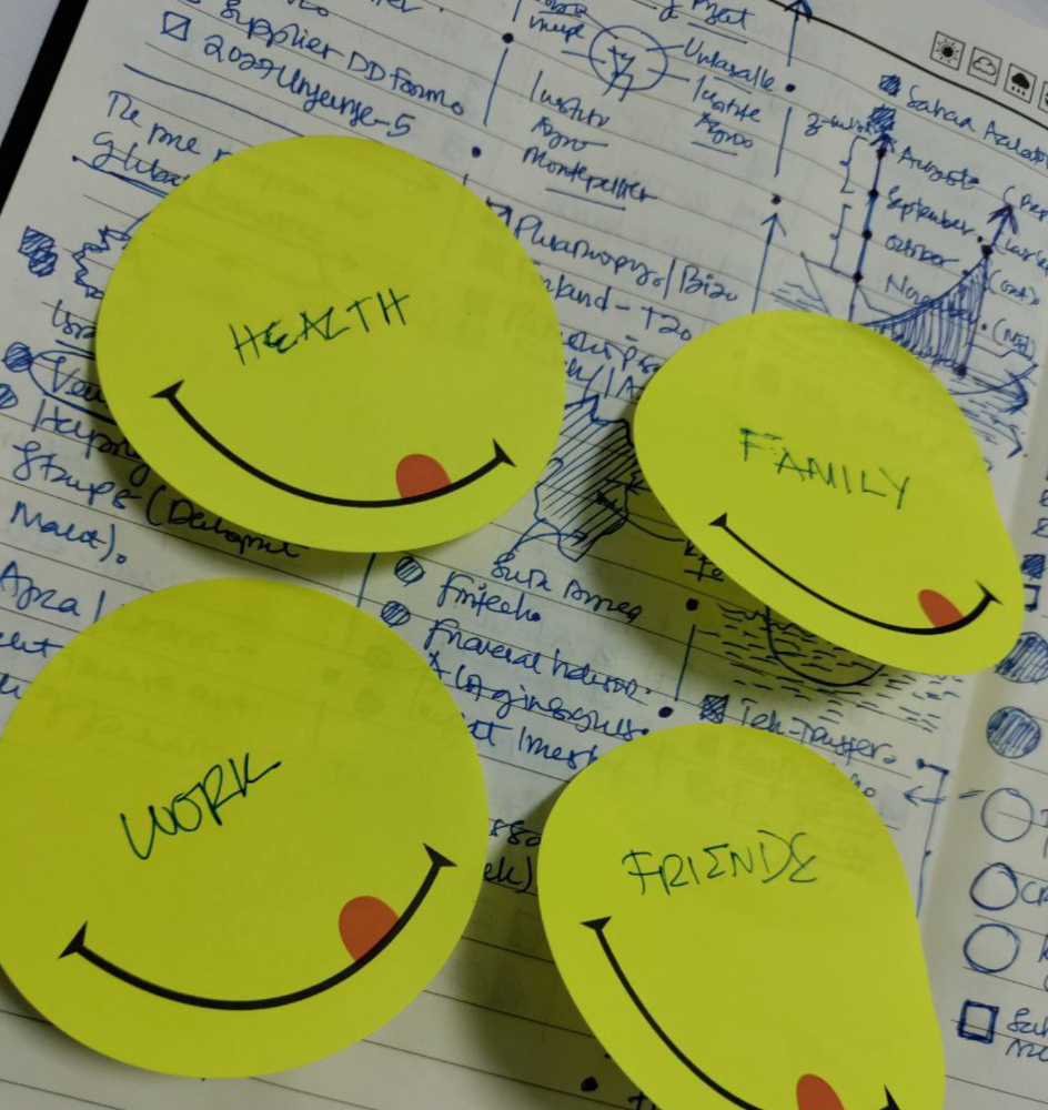
Health, Family, Work, and Friends.
The Brutal No
In a culture where people want to look good, saying "NO" to a favor request seems rude. In reality, the crime is breaking a promise. "Time Masters" have mastered "NO". More "YES" means less time, and more "NO" means more time for tasks and priorities. Brutal No doesn't mean being mean to your coworkers; it means explaining kindly and professionally that you have other priorities.
To-Do vs. MITs
Most people are productive with a routine to-do list. You can't be effective by just checking boxes on a To-do list. When was the last time you completed all of your daily tasks? Never. You must replace the to-do list with Most Important Tasks (MITs). MITs allow you to focus on the most important tasks on your list. You feel progress and accomplishment when you finish these tasks. MITs don't include ad-hoc emails, meetings, etc.
Journal Mapped
Most people don't journal or plan their day in the developing South. I've learned to plan my day in my journal over time. I have multiple sections on one page: MITs (things I want to accomplish that day), Other Activities (stuff I can postpone), Life (health, faith, and family issues), and Pop-Ups (things that just pop up). I leave the next page blank for notes. I reflected on the blocks to identify areas to improve the next day. You will have bad days, but at least you'll realize it was due to poor time management.
Buy time/delegate
Time or money? When you make enough money, you lose time to make more. The smart buy "Time." I resisted buying other people's time for years. I regret not hiring an assistant sooner. Learn to buy time from others and pay for time-consuming tasks. Sometimes you think you're saving money by doing things yourself, but you're actually losing money.
This post is a summary. See the full post here.