

More on Web3 & Crypto

Farhan Ali Khan
3 years ago
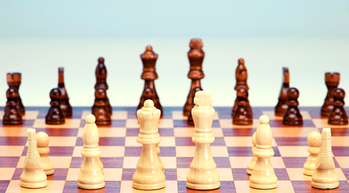
Introduction to Zero-Knowledge Proofs: The Art of Proving Without Revealing
Zero-Knowledge Proofs for Beginners
Published here originally.
Introduction
I Spy—did you play as a kid? One person chose a room object, and the other had to guess it by answering yes or no questions. I Spy was entertaining, but did you know it could teach you cryptography?
Zero Knowledge Proofs let you show your pal you know what they picked without exposing how. Math replaces electronics in this secret spy mission. Zero-knowledge proofs (ZKPs) are sophisticated cryptographic tools that allow one party to prove they have particular knowledge without revealing it. This proves identification and ownership, secures financial transactions, and more. This article explains zero-knowledge proofs and provides examples to help you comprehend this powerful technology.
What is a Proof of Zero Knowledge?
Zero-knowledge proofs prove a proposition is true without revealing any other information. This lets the prover show the verifier that they know a fact without revealing it. So, a zero-knowledge proof is like a magician's trick: the prover proves they know something without revealing how or what. Complex mathematical procedures create a proof the verifier can verify.
Want to find an easy way to test it out? Try out with tis awesome example! ZK Crush
Describe it as if I'm 5
Alex and Jack found a cave with a center entrance that only opens when someone knows the secret. Alex knows how to open the cave door and wants to show Jack without telling him.
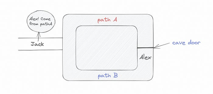
Alex and Jack name both pathways (let’s call them paths A and B).
In the first phase, Alex is already inside the cave and is free to select either path, in this case A or B.
As Alex made his decision, Jack entered the cave and asked him to exit from the B path.
Jack can confirm that Alex really does know the key to open the door because he came out for the B path and used it.
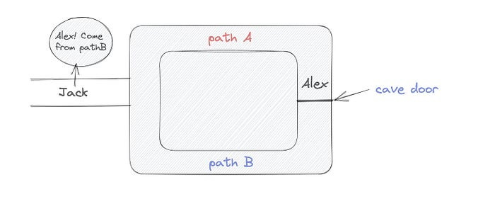
To conclude, Alex and Jack repeat:
Alex walks into the cave.
Alex follows a random route.
Jack walks into the cave.
Alex is asked to follow a random route by Jack.
Alex follows Jack's advice and heads back that way.
What is a Zero Knowledge Proof?
At a high level, the aim is to construct a secure and confidential conversation between the prover and the verifier, where the prover convinces the verifier that they have the requisite information without disclosing it. The prover and verifier exchange messages and calculate in each round of the dialogue.
The prover uses their knowledge to prove they have the information the verifier wants during these rounds. The verifier can verify the prover's truthfulness without learning more by checking the proof's mathematical statement or computation.
Zero knowledge proofs use advanced mathematical procedures and cryptography methods to secure communication. These methods ensure the evidence is authentic while preventing the prover from creating a phony proof or the verifier from extracting unnecessary information.
ZK proofs require examples to grasp. Before the examples, there are some preconditions.
Criteria for Proofs of Zero Knowledge
Completeness: If the proposition being proved is true, then an honest prover will persuade an honest verifier that it is true.
Soundness: If the proposition being proved is untrue, no dishonest prover can persuade a sincere verifier that it is true.
Zero-knowledge: The verifier only realizes that the proposition being proved is true. In other words, the proof only establishes the veracity of the proposition being supported and nothing more.
The zero-knowledge condition is crucial. Zero-knowledge proofs show only the secret's veracity. The verifier shouldn't know the secret's value or other details.
Example after example after example
To illustrate, take a zero-knowledge proof with several examples:
Initial Password Verification Example
You want to confirm you know a password or secret phrase without revealing it.
Use a zero-knowledge proof:
You and the verifier settle on a mathematical conundrum or issue, such as figuring out a big number's components.
The puzzle or problem is then solved using the hidden knowledge that you have learned. You may, for instance, utilize your understanding of the password to determine the components of a particular number.
You provide your answer to the verifier, who can assess its accuracy without knowing anything about your private data.
You go through this process several times with various riddles or issues to persuade the verifier that you actually are aware of the secret knowledge.
You solved the mathematical puzzles or problems, proving to the verifier that you know the hidden information. The proof is zero-knowledge since the verifier only sees puzzle solutions, not the secret information.
In this scenario, the mathematical challenge or problem represents the secret, and solving it proves you know it. The evidence does not expose the secret, and the verifier just learns that you know it.
My simple example meets the zero-knowledge proof conditions:
Completeness: If you actually know the hidden information, you will be able to solve the mathematical puzzles or problems, hence the proof is conclusive.
Soundness: The proof is sound because the verifier can use a publicly known algorithm to confirm that your answer to the mathematical conundrum or difficulty is accurate.
Zero-knowledge: The proof is zero-knowledge because all the verifier learns is that you are aware of the confidential information. Beyond the fact that you are aware of it, the verifier does not learn anything about the secret information itself, such as the password or the factors of the number. As a result, the proof does not provide any new insights into the secret.
Explanation #2: Toss a coin.
One coin is biased to come up heads more often than tails, while the other is fair (i.e., comes up heads and tails with equal probability). You know which coin is which, but you want to show a friend you can tell them apart without telling them.
Use a zero-knowledge proof:
One of the two coins is chosen at random, and you secretly flip it more than once.
You show your pal the following series of coin flips without revealing which coin you actually flipped.
Next, as one of the two coins is flipped in front of you, your friend asks you to tell which one it is.
Then, without revealing which coin is which, you can use your understanding of the secret order of coin flips to determine which coin your friend flipped.
To persuade your friend that you can actually differentiate between the coins, you repeat this process multiple times using various secret coin-flipping sequences.
In this example, the series of coin flips represents the knowledge of biased and fair coins. You can prove you know which coin is which without revealing which is biased or fair by employing a different secret sequence of coin flips for each round.
The evidence is zero-knowledge since your friend does not learn anything about which coin is biased and which is fair other than that you can tell them differently. The proof does not indicate which coin you flipped or how many times you flipped it.
The coin-flipping example meets zero-knowledge proof requirements:
Completeness: If you actually know which coin is biased and which is fair, you should be able to distinguish between them based on the order of coin flips, and your friend should be persuaded that you can.
Soundness: Your friend may confirm that you are correctly recognizing the coins by flipping one of them in front of you and validating your answer, thus the proof is sound in that regard. Because of this, your acquaintance can be sure that you are not just speculating or picking a coin at random.
Zero-knowledge: The argument is that your friend has no idea which coin is biased and which is fair beyond your ability to distinguish between them. Your friend is not made aware of the coin you used to make your decision or the order in which you flipped the coins. Consequently, except from letting you know which coin is biased and which is fair, the proof does not give any additional information about the coins themselves.
Figure out the prime number in Example #3.
You want to prove to a friend that you know their product n=pq without revealing p and q. Zero-knowledge proof?
Use a variant of the RSA algorithm. Method:
You determine a new number s = r2 mod n by computing a random number r.
You email your friend s and a declaration that you are aware of the values of p and q necessary for n to equal pq.
A random number (either 0 or 1) is selected by your friend and sent to you.
You send your friend r as evidence that you are aware of the values of p and q if e=0. You calculate and communicate your friend's s/r if e=1.
Without knowing the values of p and q, your friend can confirm that you know p and q (in the case where e=0) or that s/r is a legitimate square root of s mod n (in the situation where e=1).
This is a zero-knowledge proof since your friend learns nothing about p and q other than their product is n and your ability to verify it without exposing any other information. You can prove that you know p and q by sending r or by computing s/r and sending that instead (if e=1), and your friend can verify that you know p and q or that s/r is a valid square root of s mod n without learning anything else about their values. This meets the conditions of completeness, soundness, and zero-knowledge.
Zero-knowledge proofs satisfy the following:
Completeness: The prover can demonstrate this to the verifier by computing q = n/p and sending both p and q to the verifier. The prover also knows a prime number p and a factorization of n as p*q.
Soundness: Since it is impossible to identify any pair of numbers that correctly factorize n without being aware of its prime factors, the prover is unable to demonstrate knowledge of any p and q that do not do so.
Zero knowledge: The prover only admits that they are aware of a prime number p and its associated factor q, which is already known to the verifier. This is the extent of their knowledge of the prime factors of n. As a result, the prover does not provide any new details regarding n's prime factors.
Types of Proofs of Zero Knowledge
Each zero-knowledge proof has pros and cons. Most zero-knowledge proofs are:
Interactive Zero Knowledge Proofs: The prover and the verifier work together to establish the proof in this sort of zero-knowledge proof. The verifier disputes the prover's assertions after receiving a sequence of messages from the prover. When the evidence has been established, the prover will employ these new problems to generate additional responses.
Non-Interactive Zero Knowledge Proofs: For this kind of zero-knowledge proof, the prover and verifier just need to exchange a single message. Without further interaction between the two parties, the proof is established.
A statistical zero-knowledge proof is one in which the conclusion is reached with a high degree of probability but not with certainty. This indicates that there is a remote possibility that the proof is false, but that this possibility is so remote as to be unimportant.
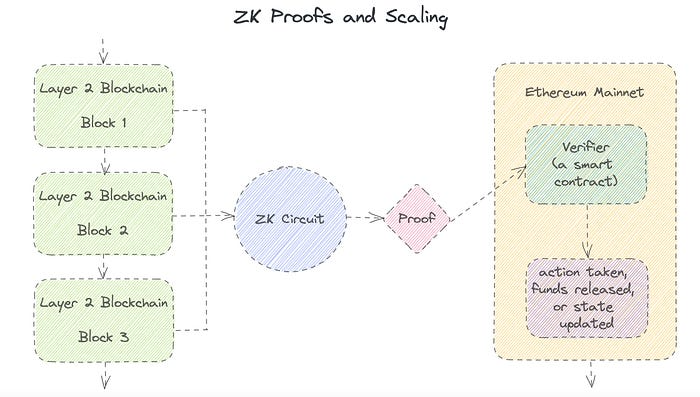
Succinct Non-Interactive Argument of Knowledge (SNARKs): SNARKs are an extremely effective and scalable form of zero-knowledge proof. They are utilized in many different applications, such as machine learning, blockchain technology, and more. Similar to other zero-knowledge proof techniques, SNARKs enable one party—the prover—to demonstrate to another—the verifier—that they are aware of a specific piece of information without disclosing any more information about that information.
The main characteristic of SNARKs is their succinctness, which refers to the fact that the size of the proof is substantially smaller than the amount of the original data being proved. Because to its high efficiency and scalability, SNARKs can be used in a wide range of applications, such as machine learning, blockchain technology, and more.
Uses for Zero Knowledge Proofs
ZKP applications include:
Verifying Identity ZKPs can be used to verify your identity without disclosing any personal information. This has uses in access control, digital signatures, and online authentication.
Proof of Ownership ZKPs can be used to demonstrate ownership of a certain asset without divulging any details about the asset itself. This has uses for protecting intellectual property, managing supply chains, and owning digital assets.
Financial Exchanges Without disclosing any details about the transaction itself, ZKPs can be used to validate financial transactions. Cryptocurrency, internet payments, and other digital financial transactions can all use this.
By enabling parties to make calculations on the data without disclosing the data itself, Data Privacy ZKPs can be used to preserve the privacy of sensitive data. Applications for this can be found in the financial, healthcare, and other sectors that handle sensitive data.
By enabling voters to confirm that their vote was counted without disclosing how they voted, elections ZKPs can be used to ensure the integrity of elections. This is applicable to electronic voting, including internet voting.
Cryptography Modern cryptography's ZKPs are a potent instrument that enable secure communication and authentication. This can be used for encrypted messaging and other purposes in the business sector as well as for military and intelligence operations.
Proofs of Zero Knowledge and Compliance
Kubernetes and regulatory compliance use ZKPs in many ways. Examples:
Security for Kubernetes ZKPs offer a mechanism to authenticate nodes without disclosing any sensitive information, enhancing the security of Kubernetes clusters. ZKPs, for instance, can be used to verify, without disclosing the specifics of the program, that the nodes in a Kubernetes cluster are running permitted software.
Compliance Inspection Without disclosing any sensitive information, ZKPs can be used to demonstrate compliance with rules like the GDPR, HIPAA, and PCI DSS. ZKPs, for instance, can be used to demonstrate that data has been encrypted and stored securely without divulging the specifics of the mechanism employed for either encryption or storage.
Access Management Without disclosing any private data, ZKPs can be used to offer safe access control to Kubernetes resources. ZKPs can be used, for instance, to demonstrate that a user has the necessary permissions to access a particular Kubernetes resource without disclosing the details of those permissions.
Safe Data Exchange Without disclosing any sensitive information, ZKPs can be used to securely transmit data between Kubernetes clusters or between several businesses. ZKPs, for instance, can be used to demonstrate the sharing of a specific piece of data between two parties without disclosing the details of the data itself.
Kubernetes deployments audited Without disclosing the specifics of the deployment or the data being processed, ZKPs can be used to demonstrate that Kubernetes deployments are working as planned. This can be helpful for auditing purposes and for ensuring that Kubernetes deployments are operating as planned.
ZKPs preserve data and maintain regulatory compliance by letting parties prove things without revealing sensitive information. ZKPs will be used more in Kubernetes as it grows.
Olga Kharif
3 years ago
A month after freezing customer withdrawals, Celsius files for bankruptcy.
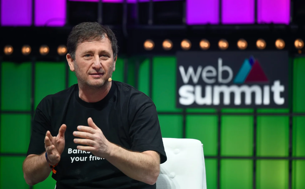
Alex Mashinsky, CEO of Celsius, speaks at Web Summit 2021 in Lisbon.
Celsius Network filed for Chapter 11 bankruptcy a month after freezing customer withdrawals, joining other crypto casualties.
Celsius took the step to stabilize its business and restructure for all stakeholders. The filing was done in the Southern District of New York.
The company, which amassed more than $20 billion by offering 18% interest on cryptocurrency deposits, paused withdrawals and other functions in mid-June, citing "extreme market conditions."
As the Fed raises interest rates aggressively, it hurts risk sentiment and squeezes funding costs. Voyager Digital Ltd. filed for Chapter 11 bankruptcy this month, and Three Arrows Capital has called in liquidators.
Celsius called the pause "difficult but necessary." Without the halt, "the acceleration of withdrawals would have allowed certain customers to be paid in full while leaving others to wait for Celsius to harvest value from illiquid or longer-term asset deployment activities," it said.
Celsius declined to comment. CEO Alex Mashinsky said the move will strengthen the company's future.
The company wants to keep operating. It's not requesting permission to allow customer withdrawals right now; Chapter 11 will handle customer claims. The filing estimates assets and liabilities between $1 billion and $10 billion.
Celsius is advised by Kirkland & Ellis, Centerview Partners, and Alvarez & Marsal.
Yield-promises
Celsius promised 18% returns on crypto loans. It lent those coins to institutional investors and participated in decentralized-finance apps.
When TerraUSD (UST) and Luna collapsed in May, Celsius pulled its funds from Terra's Anchor Protocol, which offered 20% returns on UST deposits. Recently, another large holding, staked ETH, or stETH, which is tied to Ether, became illiquid and discounted to Ether.
The lender is one of many crypto companies hurt by risky bets in the bear market. Also, Babel halted withdrawals. Voyager Digital filed for bankruptcy, and crypto hedge fund Three Arrows Capital filed for Chapter 15 bankruptcy.
According to blockchain data and tracker Zapper, Celsius repaid all of its debt in Aave, Compound, and MakerDAO last month.
Celsius charged Symbolic Capital Partners Ltd. 2,000 Ether as collateral for a cash loan on June 13. According to company filings, Symbolic was charged 2,545.25 Ether on June 11.
In July 6 filings, it said it reshuffled its board, appointing two new members and firing others.

Sam Bourgi
3 years ago
NFT was used to serve a restraining order on an anonymous hacker.
The international law firm Holland & Knight used an NFT built and airdropped by its asset recovery team to serve a defendant in a hacking case.
The law firms Holland & Knight and Bluestone used a nonfungible token to serve a defendant in a hacking case with a temporary restraining order, marking the first documented legal process assisted by an NFT.
The so-called "service token" or "service NFT" was served to an unknown defendant in a hacking case involving LCX, a cryptocurrency exchange based in Liechtenstein that was hacked for over $8 million in January. The attack compromised the platform's hot wallets, resulting in the loss of Ether (ETH), USD Coin (USDC), and other cryptocurrencies, according to Cointelegraph at the time.
On June 7, LCX claimed that around 60% of the stolen cash had been frozen, with investigations ongoing in Liechtenstein, Ireland, Spain, and the United States. Based on a court judgment from the New York Supreme Court, Centre Consortium, a company created by USDC issuer Circle and crypto exchange Coinbase, has frozen around $1.3 million in USDC.
The monies were laundered through Tornado Cash, according to LCX, but were later tracked using "algorithmic forensic analysis." The organization was also able to identify wallets linked to the hacker as a result of the investigation.
In light of these findings, the law firms representing LCX, Holland & Knight and Bluestone, served the unnamed defendant with a temporary restraining order issued on-chain using an NFT. According to LCX, this system "was allowed by the New York Supreme Court and is an example of how innovation can bring legitimacy and transparency to a market that some say is ungovernable."
You might also like

Sad NoCoiner
3 years ago
Two Key Money Principles You Should Understand But Were Never Taught
Prudence is advised. Be debt-free. Be frugal. Spend less.
This advice sounds nice, but it rarely works.
Most people never learn these two money rules. Both approaches will impact how you see personal finance.
It may safeguard you from inflation or the inability to preserve money.
Let’s dive in.
#1: Making long-term debt your ally
High-interest debt hurts consumers. Many credit cards carry 25% yearly interest (or more), so always pay on time. Otherwise, you’re losing money.
Some low-interest debt is good. Especially when buying an appreciating asset with borrowed money.
Inflation helps you.
If you borrow $800,000 at 3% interest and invest it at 7%, you'll make $32,000 (4%).
As money loses value, fixed payments get cheaper. Your assets' value and cash flow rise.
The never-in-debt crowd doesn't know this. They lose money paying off mortgages and low-interest loans early when they could have bought assets instead.
#2: How To Buy Or Build Assets To Make Inflation Irrelevant
Dozens of studies demonstrate actual wage growth is static; $2.50 in 1964 was equivalent to $22.65 now.
These reports never give solutions unless they're selling gold.
But there is one.
Assets beat inflation.
$100 invested into the S&P 500 would have an inflation-adjusted return of 17,739.30%.
Likewise, you can build assets from nothing. Doing is easy and quick. The returns can boost your income by 10% or more.
The people who obsess over inflation inadvertently make the problem worse for themselves. They wait for The Big Crash to buy assets. Or they moan about debt clocks and spending bills instead of seeking a solution.
Conclusion
Being ultra-prudent is like playing golf with a putter to avoid hitting the ball into the water. Sure, you might not slice a drive into the pond. But, you aren’t going to play well either. Or have very much fun.
Money has rules.
Avoiding debt or investment risks will limit your rewards. Long-term, being too cautious hurts your finances.
Disclaimer: This article is for entertainment purposes only. It is not financial advice, always do your own research.

The Secret Developer
3 years ago
What Elon Musk's Take on Bitcoin Teaches Us
Tesla Q2 earnings revealed unethical dealings.
As of end of Q2, we have converted approximately 75% of our Bitcoin purchases into fiat currency
That’s OK then, isn’t it?
Elon Musk, Tesla's CEO, is now untrustworthy.
It’s not about infidelity, it’s about doing the right thing
And what can we learn?
The Opening Remark
Musk tweets on his (and Tesla's) future goals.
Don’t worry, I’m not expecting you to read it.
What's crucial?
Tesla will not be selling any Bitcoin
The Situation as It Develops
2021 Tesla spent $1.5 billion on Bitcoin. In 2022, they sold 75% of the ownership for $946 million.
That’s a little bit of a waste of money, right?
Musk predicted the reverse would happen.
What gives? Why would someone say one thing, then do the polar opposite?
The Justification For Change
Tesla's public. They must follow regulations. When a corporation trades, they must record what happens.
At least this keeps Musk some way in line.
We now understand Musk and Tesla's actions.
Musk claimed that Tesla sold bitcoins to maximize cash given the unpredictability of COVID lockdowns in China.
Tesla may buy Bitcoin in the future, he said.
That’s fine then. He’s not knocking the NFT at least.
Tesla has moved investments into cash due to China lockdowns.
That doesn’t explain the 180° though
Musk's Tweet isn't company policy. Therefore, the CEO's change of heart reflects the organization. Look.
That's okay, since
Leaders alter their positions when circumstances change.
Leaders must adapt to their surroundings. This isn't embarrassing; it's a leadership prerequisite.
Yet
The Man
Someone stated if you're not in the office full-time, you need to explain yourself. He doesn't treat his employees like adults.
This is the individual mentioned in the quote.
If Elon was not happy, you knew it. Things could get nasty
also, He fired his helper for requesting a raise.
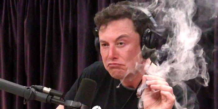
This public persona isn't good. Without mentioning his disastrous performances on Twitter (pedo dude) or Joe Rogan. This image sums up the odd Podcast appearance:
Which describes the man.
I wouldn’t trust this guy to feed a cat
What we can discover
When Musk's company bet on Bitcoin, what happened?
Exactly what we would expect
The company's position altered without the CEO's awareness. He seems uncaring.
This article is about how something happened, not what happened. Change of thinking requires contrition.
This situation is about a lack of respect- although you might argue that followers on Twitter don’t deserve any
Tesla fans call the sale a great move.
It's absurd.
As you were, then.
Conclusion
Good luck if you gamble.
When they pay off, congrats!
When wrong, admit it.
You must take chances if you want to succeed.
Risks don't always pay off.
Mr. Musk lacks insight and charisma to combine these two attributes.
I don’t like him, if you hadn’t figured.
It’s probably all of the cheating.

Taher Batterywala
3 years ago
Do You Have Focus Issues? Use These 5 Simple Habits
Many can't concentrate. The first 20% of the day isn't optimized.
Elon Musk, Tony Robbins, and Bill Gates share something:
Morning Routines.
A repeatable morning ritual saves time.
The result?
Time for hobbies.
I'll discuss 5 easy morning routines you can use.
1. Stop pressing snooze
Waking up starts the day. You disrupt your routine by hitting snooze.
One sleep becomes three. Your morning routine gets derailed.
Fix it:
Hide your phone. This disables snooze and wakes you up.
Once awake, staying awake is 10x easier. Simple trick, big results.
2. Drink water
Chronic dehydration is common. Mostly urban, air-conditioned workers/residents.
2% cerebral dehydration causes short-term memory loss.
Dehydration shrinks brain cells.
Drink 3-4 liters of water daily to avoid this.
3. Improve your focus
How to focus better?
Meditation.
Improve your mood
Enhance your memory
increase mental clarity
Reduce blood pressure and stress
Headspace helps with the habit.
Here's a meditation guide.
Sit comfortably
Shut your eyes.
Concentrate on your breathing
Breathe in through your nose
Breathe out your mouth.
5 in, 5 out.
Repeat for 1 to 20 minutes.
Here's a beginner's video:
4. Workout
Exercise raises:
Mental Health
Effort levels
focus and memory
15-60 minutes of fun:
Exercise Lifting
Running
Walking
Stretching and yoga
This helps you now and later.
5. Keep a journal
You have countless thoughts daily. Many quietly steal your focus.
Here’s how to clear these:
Write for 5-10 minutes.
You'll gain 2x more mental clarity.
Recap
5 morning practices for 5x more productivity:
Say no to snoozing
Hydrate
Improve your focus
Exercise
Journaling
Conclusion
One step starts a thousand-mile journey. Try these easy yet effective behaviors if you have trouble concentrating or have too many thoughts.
Start with one of these behaviors, then add the others. Its astonishing results are instant.