

:max_bytes(150000):strip_icc():format(webp)/adam_hayes-5bfc262a46e0fb005118b414.jpg)
Bernard Lawrence "Bernie" Madoff, the largest Ponzi scheme in history
Madoff who?
Bernie Madoff ran the largest Ponzi scheme in history, defrauding thousands of investors over at least 17 years, and possibly longer. He pioneered electronic trading and chaired Nasdaq in the 1990s. On April 14, 2021, he died while serving a 150-year sentence for money laundering, securities fraud, and other crimes.
Understanding Madoff
Madoff claimed to generate large, steady returns through a trading strategy called split-strike conversion, but he simply deposited client funds into a single bank account and paid out existing clients. He funded redemptions by attracting new investors and their capital, but the market crashed in late 2008. He confessed to his sons, who worked at his firm, on Dec. 10, 2008. Next day, they turned him in. The fund reported $64.8 billion in client assets.
Madoff pleaded guilty to 11 federal felony counts, including securities fraud, wire fraud, mail fraud, perjury, and money laundering. Ponzi scheme became a symbol of Wall Street's greed and dishonesty before the financial crisis. Madoff was sentenced to 150 years in prison and ordered to forfeit $170 billion, but no other Wall Street figures faced legal ramifications.
Bernie Madoff's Brief Biography
Bernie Madoff was born in Queens, New York, on April 29, 1938. He began dating Ruth (née Alpern) when they were teenagers. Madoff told a journalist by phone from prison that his father's sporting goods store went bankrupt during the Korean War: "You watch your father, who you idolize, build a big business and then lose everything." Madoff was determined to achieve "lasting success" like his father "whatever it took," but his career had ups and downs.
Early Madoff investments
At 22, he started Bernard L. Madoff Investment Securities LLC. First, he traded penny stocks with $5,000 he earned installing sprinklers and as a lifeguard. Family and friends soon invested with him. Madoff's bets soured after the "Kennedy Slide" in 1962, and his father-in-law had to bail him out.
Madoff felt he wasn't part of the Wall Street in-crowd. "We weren't NYSE members," he told Fishman. "It's obvious." According to Madoff, he was a scrappy market maker. "I was happy to take the crumbs," he told Fishman, citing a client who wanted to sell eight bonds; a bigger firm would turn it down.
Recognition
Success came when he and his brother Peter built electronic trading capabilities, or "artificial intelligence," that attracted massive order flow and provided market insights. "I had all these major banks coming down, entertaining me," Madoff told Fishman. "It was mind-bending."
By the late 1980s, he and four other Wall Street mainstays processed half of the NYSE's order flow. Controversially, he paid for much of it, and by the late 1980s, Madoff was making in the vicinity of $100 million a year. He was Nasdaq chairman from 1990 to 1993.
Madoff's Ponzi scheme
It is not certain exactly when Madoff's Ponzi scheme began. He testified in court that it began in 1991, but his account manager, Frank DiPascali, had been at the firm since 1975.
Why Madoff did the scheme is unclear. "I had enough money to support my family's lifestyle. "I don't know why," he told Fishman." Madoff could have won Wall Street's respect as a market maker and electronic trading pioneer.
Madoff told Fishman he wasn't solely responsible for the fraud. "I let myself be talked into something, and that's my fault," he said, without saying who convinced him. "I thought I could escape eventually. I thought it'd be quick, but I couldn't."
Carl Shapiro, Jeffry Picower, Stanley Chais, and Norm Levy have been linked to Bernard L. Madoff Investment Securities LLC for years. Madoff's scheme made these men hundreds of millions of dollars in the 1960s and 1970s.
Madoff told Fishman, "Everyone was greedy, everyone wanted to go on." He says the Big Four and others who pumped client funds to him, outsourcing their asset management, must have suspected his returns or should have. "How can you make 15%-18% when everyone else is making less?" said Madoff.
How Madoff Got Away with It for So Long
Madoff's high returns made clients look the other way. He deposited their money in a Chase Manhattan Bank account, which merged to become JPMorgan Chase & Co. in 2000. The bank may have made $483 million from those deposits, so it didn't investigate.
When clients redeemed their investments, Madoff funded the payouts with new capital he attracted by promising unbelievable returns and earning his victims' trust. Madoff created an image of exclusivity by turning away clients. This model let half of Madoff's investors profit. These investors must pay into a victims' fund for defrauded investors.
Madoff wooed investors with his philanthropy. He defrauded nonprofits, including the Elie Wiesel Foundation for Peace and Hadassah. He approached congregants through his friendship with J. Ezra Merkin, a synagogue officer. Madoff allegedly stole $1 billion to $2 billion from his investors.
Investors believed Madoff for several reasons:
- His public portfolio seemed to be blue-chip stocks.
- His returns were high (10-20%) but consistent and not outlandish. In a 1992 interview with Madoff, the Wall Street Journal reported: "[Madoff] insists the returns were nothing special, given that the S&P 500-stock index returned 16.3% annually from 1982 to 1992. 'I'd be surprised if anyone thought matching the S&P over 10 years was remarkable,' he says.
- "He said he was using a split-strike collar strategy. A collar protects underlying shares by purchasing an out-of-the-money put option.
SEC inquiry
The Securities and Exchange Commission had been investigating Madoff and his securities firm since 1999, which frustrated many after he was prosecuted because they felt the biggest damage could have been prevented if the initial investigations had been rigorous enough.
Harry Markopolos was a whistleblower. In 1999, he figured Madoff must be lying in an afternoon. The SEC ignored his first Madoff complaint in 2000.
Markopolos wrote to the SEC in 2005: "The largest Ponzi scheme is Madoff Securities. This case has no SEC reward, so I'm turning it in because it's the right thing to do."
Many believed the SEC's initial investigations could have prevented Madoff's worst damage.
Markopolos found irregularities using a "Mosaic Method." Madoff's firm claimed to be profitable even when the S&P fell, which made no mathematical sense given what he was investing in. Markopolos said Madoff Securities' "undisclosed commissions" were the biggest red flag (1 percent of the total plus 20 percent of the profits).
Markopolos concluded that "investors don't know Bernie Madoff manages their money." Markopolos learned Madoff was applying for large loans from European banks (seemingly unnecessary if Madoff's returns were high).
The regulator asked Madoff for trading account documentation in 2005, after he nearly went bankrupt due to redemptions. The SEC drafted letters to two of the firms on his six-page list but didn't send them. Diana Henriques, author of "The Wizard of Lies: Bernie Madoff and the Death of Trust," documents the episode.
In 2008, the SEC was criticized for its slow response to Madoff's fraud.
Confession, sentencing of Bernie Madoff
Bernard L. Madoff Investment Securities LLC reported 5.6% year-to-date returns in November 2008; the S&P 500 fell 39%. As the selling continued, Madoff couldn't keep up with redemption requests, and on Dec. 10, he confessed to his sons Mark and Andy, who worked at his firm. "After I told them, they left, went to a lawyer, who told them to turn in their father, and I never saw them again. 2008-12-11: Bernie Madoff arrested.
Madoff insists he acted alone, but several of his colleagues were jailed. Mark Madoff died two years after his father's fraud was exposed. Madoff's investors committed suicide. Andy Madoff died of cancer in 2014.
2009 saw Madoff's 150-year prison sentence and $170 billion forfeiture. Marshals sold his three homes and yacht. Prisoner 61727-054 at Butner Federal Correctional Institution in North Carolina.
Madoff's lawyers requested early release on February 5, 2020, claiming he has a terminal kidney disease that may kill him in 18 months. Ten years have passed since Madoff's sentencing.
Bernie Madoff's Ponzi scheme aftermath
The paper trail of victims' claims shows Madoff's complexity and size. Documents show Madoff's scam began in the 1960s. His final account statements show $47 billion in "profit" from fake trades and shady accounting.
Thousands of investors lost their life savings, and multiple stories detail their harrowing loss.
Irving Picard, a New York lawyer overseeing Madoff's bankruptcy, has helped investors. By December 2018, Picard had recovered $13.3 billion from Ponzi scheme profiteers.
A Madoff Victim Fund (MVF) was created in 2013 to help compensate Madoff's victims, but the DOJ didn't start paying out the $4 billion until late 2017. Richard Breeden, a former SEC chair who oversees the fund, said thousands of claims were from "indirect investors"
Breeden and his team had to reject many claims because they weren't direct victims. Breeden said he based most of his decisions on one simple rule: Did the person invest more than they withdrew? Breeden estimated 11,000 "feeder" investors.
Breeden wrote in a November 2018 update for the Madoff Victim Fund, "We've paid over 27,300 victims 56.65% of their losses, with thousands more to come." In December 2018, 37,011 Madoff victims in the U.S. and around the world received over $2.7 billion. Breeden said the fund expected to make "at least one more significant distribution in 2019"
This post is a summary. Read full article here
More on Economics & Investing

Sylvain Saurel
3 years ago
A student trader from the United States made $110 million in one month and rose to prominence on Wall Street.
Genius or lucky?
From the title, you might think I'm selling advertising for a financial influencer, a dubious trading site, or a training organization to attract clients. I'm suspicious. Better safe than sorry.
But not here.
Jake Freeman, 20, made $110 million in a month, according to the Financial Times. At 18, he ran for president. He made his name in markets, not politics. Two years later, he's Wall Street's prince. Interview requests flood the prodigy.
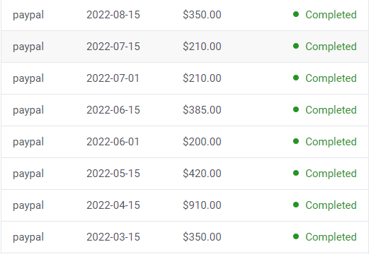
Jake Freeman bought 5 million Bed Bath & Beyond Group shares for $5.5 in July 2022 and sold them for $27 a month later. He thought the stock might double. Since speculation died down, he sold well. The stock fell 40.5% to 11 dollars on Friday, 19 August 2022. On August 22, 2022, it fell 16% to $9.
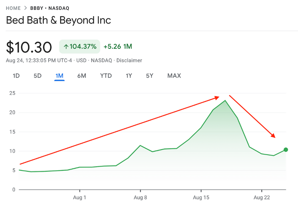
Smallholders have been buying the stock for weeks and will lose heavily if it falls further. Bed Bath & Beyond is the second most popular stock after Foot Locker, ahead of GameStop and Apple.
Jake Freeman earned $110 million thanks to a significant stock market flurry.
Online broker customers aren't the only ones with jitters. By June 2022, Ken Griffin's Citadel and Stephen Mandel's Lone Pine Capital held nearly a third of the company's capital. Did big managers sell before the stock plummeted?
Recent stock movements (derivatives) and rumors could prompt a SEC investigation.
Jake Freeman wrote to the board of directors after his investment to call for a turnaround, given the company's persistent problems and short sellers. The bathroom and kitchen products distribution group's stock soared in July 2022 due to renewed buying by private speculators, who made it one of their meme stocks with AMC and GameStop.
Second-quarter 2022 results and financial health worsened. He didn't celebrate his miraculous operation in a nightclub. He told a British newspaper, "I'm shocked." His parents dined in New York. He returned to Los Angeles to study math and economics.
Jake Freeman founded Freeman Capital Management with his savings and $25 million from family, friends, and acquaintances. They are the ones who are entitled to the $110 million he raised in one month. Will his investors pocket and withdraw all or part of their profits or will they trust the young prodigy for new stunts on Wall Street?
His operation should attract new clients. Well-known hedge funds may hire him.
Jake Freeman didn't listen to gurus or former traders. At 17, he interned at a quantitative finance and derivatives hedge fund, Volaris. At 13, he began investing with his pharmaceutical executive uncle. All countries have increased their Google searches for the young trader in the last week.
Naturally, his success has inspired resentment.
His success stirs jealousy, and he's attacked on social media. On Reddit, people who lost money on Bed Bath & Beyond, Jake Freeman's fortune, are mourning.
Several conspiracy theories circulate about him, including that he doesn't exist or is working for a Taiwanese amusement park.
If all 20 million American students had the same trading skills, they would have generated $1.46 trillion. Jake Freeman is unique. Apprentice traders' careers are often short, disillusioning, and tragic.
Two years ago, 20-year-old Robinhood client Alexander Kearns committed suicide after losing $750,000 trading options. Great traders start young. Michael Platt of BlueCrest invested in British stocks at age 12 under his grandmother's supervision and made a £30,000 fortune. Paul Tudor Jones started trading before he turned 18 with his uncle. Warren Buffett, at age 10, was discussing investments with Goldman Sachs' head. Oracle of Omaha tells all.

Sofien Kaabar, CFA
2 years ago
Innovative Trading Methods: The Catapult Indicator
Python Volatility-Based Catapult Indicator
As a catapult, this technical indicator uses three systems: Volatility (the fulcrum), Momentum (the propeller), and a Directional Filter (Acting as the support). The goal is to get a signal that predicts volatility acceleration and direction based on historical patterns. We want to know when the market will move. and where. This indicator outperforms standard indicators.
Knowledge must be accessible to everyone. This is why my new publications Contrarian Trading Strategies in Python and Trend Following Strategies in Python now include free PDF copies of my first three books (Therefore, purchasing one of the new books gets you 4 books in total). GitHub-hosted advanced indications and techniques are in the two new books above.
The Foundation: Volatility
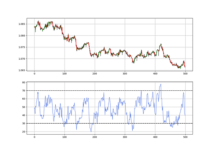
The Catapult predicts significant changes with the 21-period Relative Volatility Index.
The Average True Range, Mean Absolute Deviation, and Standard Deviation all assess volatility. Standard Deviation will construct the Relative Volatility Index.
Standard Deviation is the most basic volatility. It underpins descriptive statistics and technical indicators like Bollinger Bands. Before calculating Standard Deviation, let's define Variance.
Variance is the squared deviations from the mean (a dispersion measure). We take the square deviations to compel the distance from the mean to be non-negative, then we take the square root to make the measure have the same units as the mean, comparing apples to apples (mean to standard deviation standard deviation). Variance formula:
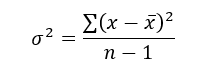
As stated, standard deviation is:
# The function to add a number of columns inside an array
def adder(Data, times):

    for i in range(1, times + 1):

        new_col = np.zeros((len(Data), 1), dtype = float)
        Data = np.append(Data, new_col, axis = 1)

    return Data

# The function to delete a number of columns starting from an index
def deleter(Data, index, times):

    for i in range(1, times + 1):

        Data = np.delete(Data, index, axis = 1)

    return Data

# The function to delete a number of rows from the beginning
def jump(Data, jump):

    Data = Data[jump:, ]

    return Data

# Example of adding 3 empty columns to an array
my_ohlc_array = adder(my_ohlc_array, 3)

# Example of deleting the 2 columns after the column indexed at 3
my_ohlc_array = deleter(my_ohlc_array, 3, 2)

# Example of deleting the first 20 rows
my_ohlc_array = jump(my_ohlc_array, 20)

# Remember, OHLC is an abbreviation of Open, High, Low, and Close and it refers to the standard historical data file

def volatility(Data, lookback, what, where):

  for i in range(len(Data)):

     try:

        Data[i, where] = (Data[i - lookback + 1:i + 1, what].std())
     except IndexError:
        pass

  return Data
The RSI is the most popular momentum indicator, and for good reason—it excels in range markets. Its 0–100 range simplifies interpretation. Fame boosts its potential.
The more traders and portfolio managers look at the RSI, the more people will react to its signals, pushing market prices. Technical Analysis is self-fulfilling, therefore this theory is obvious yet unproven.
RSI is determined simply. Start with one-period pricing discrepancies. We must remove each closing price from the previous one. We then divide the smoothed average of positive differences by the smoothed average of negative differences. The RSI algorithm converts the Relative Strength from the last calculation into a value between 0 and 100.
def ma(Data, lookback, close, where):

    Data = adder(Data, 1)

    for i in range(len(Data)):

            try:
                Data[i, where] = (Data[i - lookback + 1:i + 1, close].mean())

            except IndexError:
                pass

    # Cleaning
    Data = jump(Data, lookback)

    return Data
def ema(Data, alpha, lookback, what, where):

    alpha = alpha / (lookback + 1.0)
    beta  = 1 - alpha

    # First value is a simple SMA
    Data = ma(Data, lookback, what, where)

    # Calculating first EMA
    Data[lookback + 1, where] = (Data[lookback + 1, what] * alpha) + (Data[lookback, where] * beta)

    # Calculating the rest of EMA
    for i in range(lookback + 2, len(Data)):
            try:
                Data[i, where] = (Data[i, what] * alpha) + (Data[i - 1, where] * beta)

            except IndexError:
                pass

    return Datadef rsi(Data, lookback, close, where, width = 1, genre = 'Smoothed'):

    # Adding a few columns
    Data = adder(Data, 7)

    # Calculating Differences
    for i in range(len(Data)):

        Data[i, where] = Data[i, close] - Data[i - width, close]

    # Calculating the Up and Down absolute values
    for i in range(len(Data)):

        if Data[i, where] > 0:

            Data[i, where + 1] = Data[i, where]

        elif Data[i, where] < 0:

            Data[i, where + 2] = abs(Data[i, where])

    # Calculating the Smoothed Moving Average on Up and Down
    absolute values

    lookback = (lookback * 2) - 1 # From exponential to smoothed
    Data = ema(Data, 2, lookback, where + 1, where + 3)
    Data = ema(Data, 2, lookback, where + 2, where + 4)

    # Calculating the Relative Strength
    Data[:, where + 5] = Data[:, where + 3] / Data[:, where + 4]

    # Calculate the Relative Strength Index
    Data[:, where + 6] = (100 - (100 / (1 + Data[:, where + 5])))

    # Cleaning
    Data = deleter(Data, where, 6)
    Data = jump(Data, lookback)

    return Data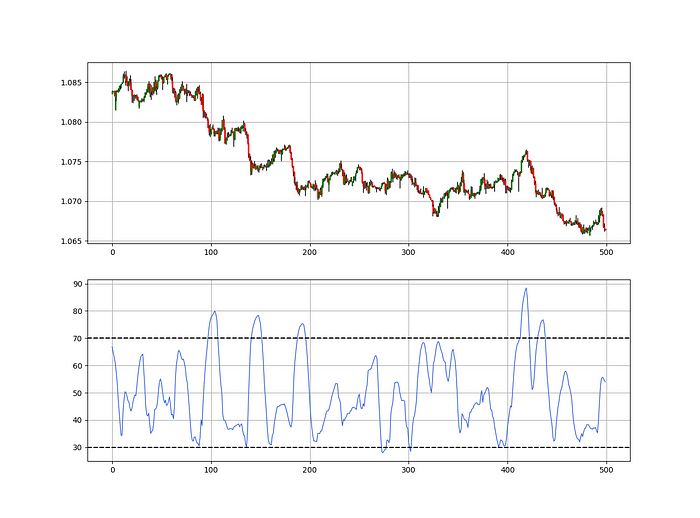
def relative_volatility_index(Data, lookback, close, where):

    # Calculating Volatility
    Data = volatility(Data, lookback, close, where)

    # Calculating the RSI on Volatility
    Data = rsi(Data, lookback, where, where + 1)

    # Cleaning
    Data = deleter(Data, where, 1)

    return Data
The Arm Section: Speed
The Catapult predicts momentum direction using the 14-period Relative Strength Index.
As a reminder, the RSI ranges from 0 to 100. Two levels give contrarian signals:
A positive response is anticipated when the market is deemed to have gone too far down at the oversold level 30, which is 30.
When the market is deemed to have gone up too much, at overbought level 70, a bearish reaction is to be expected.
Comparing the RSI to 50 is another intriguing use. RSI above 50 indicates bullish momentum, while below 50 indicates negative momentum.
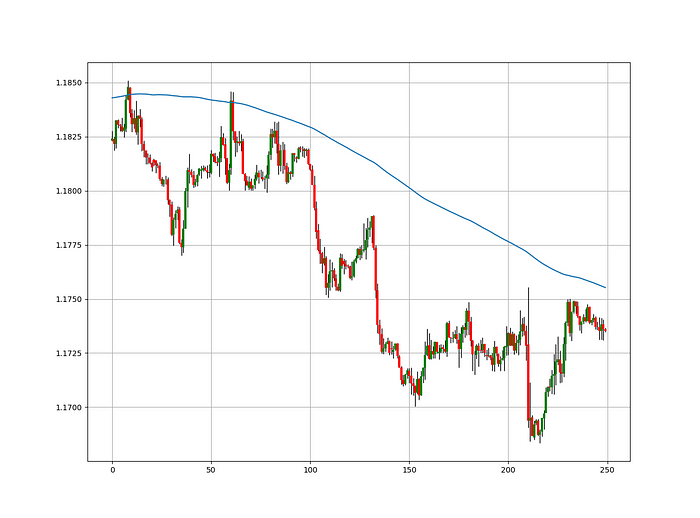
The direction-finding filter in the frame
The Catapult's directional filter uses the 200-period simple moving average to keep us trending. This keeps us sane and increases our odds.
Moving averages confirm and ride trends. Its simplicity and track record of delivering value to analysis make them the most popular technical indicator. They help us locate support and resistance, stops and targets, and the trend. Its versatility makes them essential trading tools.
This is the plain mean, employed in statistics and everywhere else in life. Simply divide the number of observations by their total values. Mathematically, it's:
We defined the moving average function above. Create the Catapult indication now.
Indicator of the Catapult
The indicator is a healthy mix of the three indicators:
The first trigger will be provided by the 21-period Relative Volatility Index, which indicates that there will now be above average volatility and, as a result, it is possible for a directional shift.
If the reading is above 50, the move is likely bullish, and if it is below 50, the move is likely bearish, according to the 14-period Relative Strength Index, which indicates the likelihood of the direction of the move.
The likelihood of the move's direction will be strengthened by the 200-period simple moving average. When the market is above the 200-period moving average, we can infer that bullish pressure is there and that the upward trend will likely continue. Similar to this, if the market falls below the 200-period moving average, we recognize that there is negative pressure and that the downside is quite likely to continue.
lookback_rvi = 21
lookback_rsi = 14
lookback_ma = 200
my_data = ma(my_data, lookback_ma, 3, 4)
my_data = rsi(my_data, lookback_rsi, 3, 5)
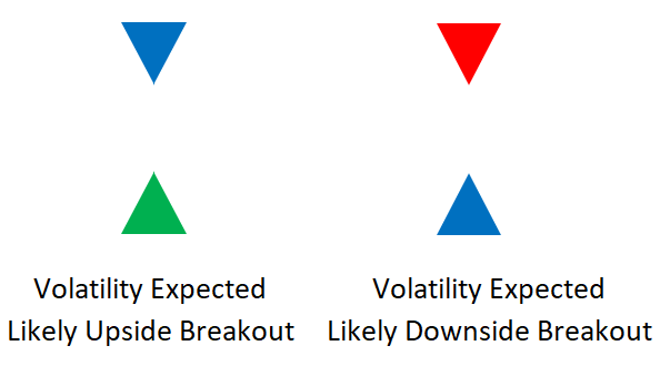
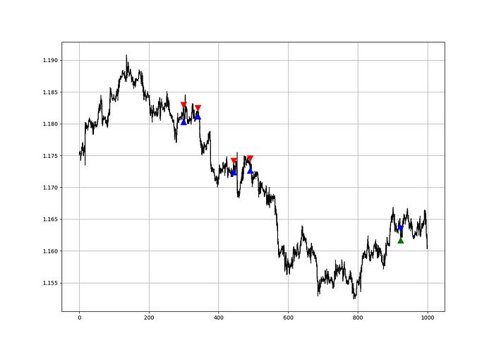
my_data = relative_volatility_index(my_data, lookback_rvi, 3, 6)Two-handled overlay indicator Catapult. The first exhibits blue and green arrows for a buy signal, and the second shows blue and red for a sell signal.
The chart below shows recent EURUSD hourly values.
def signal(Data, rvi_col, signal):

    Data = adder(Data, 10)

    for i in range(len(Data)):

        if Data[i,     rvi_col] < 30 and \
           Data[i - 1, rvi_col] > 30 and \
           Data[i - 2, rvi_col] > 30 and \
           Data[i - 3, rvi_col] > 30 and \
           Data[i - 4, rvi_col] > 30 and \
           Data[i - 5, rvi_col] > 30:

               Data[i, signal] = 1

    return Data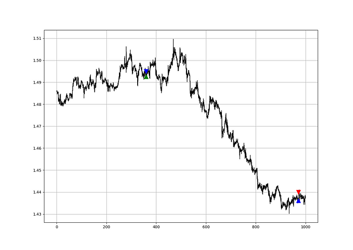
Signals are straightforward. The indicator can be utilized with other methods.
my_data = signal(my_data, 6, 7)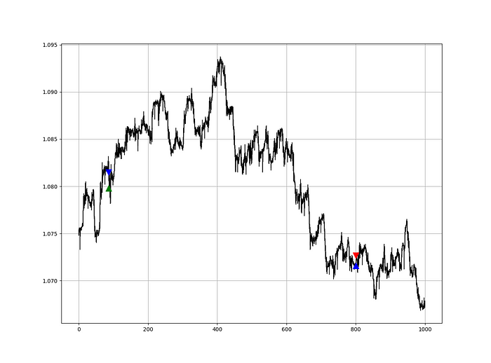
Lumiwealth shows how to develop all kinds of algorithms. I recommend their hands-on courses in algorithmic trading, blockchain, and machine learning.
Summary
To conclude, my goal is to contribute to objective technical analysis, which promotes more transparent methods and strategies that must be back-tested before implementation. Technical analysis will lose its reputation as subjective and unscientific.
After you find a trading method or approach, follow these steps:
Put emotions aside and adopt an analytical perspective.
Test it in the past in conditions and simulations taken from real life.
Try improving it and performing a forward test if you notice any possibility.
Transaction charges and any slippage simulation should always be included in your tests.
Risk management and position sizing should always be included in your tests.
After checking the aforementioned, monitor the plan because market dynamics may change and render it unprofitable.

Desiree Peralta
3 years ago
How to Use the 2023 Recession to Grow Your Wealth Exponentially
This season's three best money moves.

“Millionaires are made in recessions.” — Time Capital
We're in a serious downturn, whether or not we're in a recession.
97% of business owners are decreasing costs by more than 10%, and all markets are down 30%.
If you know what you're doing and analyze the markets correctly, this is your chance to become a millionaire.
In any recession, there are always excellent possibilities to seize. Real estate, crypto, stocks, enterprises, etc.
What you do with your money could influence your future riches.
This article analyzes the three key markets, their circumstances for 2023, and how to profit from them.
Ways to make money on the stock market.
If you're conservative like me, you should invest in an index fund. Most of these funds are down 10-30% of ATH:
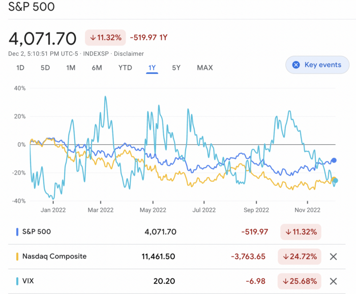
In earlier recessions, most money index funds lost 20%. After this downturn, they grew and passed the ATH in subsequent months.
Now is the greatest moment to invest in index funds to grow your money in a low-risk approach and make 20%.
If you want to be risky but wise, pick companies that will get better next year but are struggling now.
Even while we can't be 100% confident of a company's future performance, we know some are strong and will have a fantastic year.
Microsoft (down 22%), JPMorgan Chase (15.6%), Amazon (45%), and Disney (33.8%).
These firms give dividends, so you can earn passively while you wait.
So I consider that a good strategy to make wealth in the current stock market is to create two portfolios: one based on index funds to earn 10% to 20% profit when the corrections end, and the other based on individual stocks of popular and strong companies to earn 20%-30% return and dividends while you wait.
How to profit from the downturn in the real estate industry.
With rising mortgage rates, it's the worst moment to buy a home if you don't want to be eaten by banks. In the U.S., interest rates are double what they were three years ago, so buying now looks foolish.
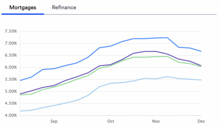
Due to these rates, property prices are falling, but that won't last long since individuals will take advantage.
According to historical data, now is the ideal moment to buy a house for the next five years and perhaps forever.
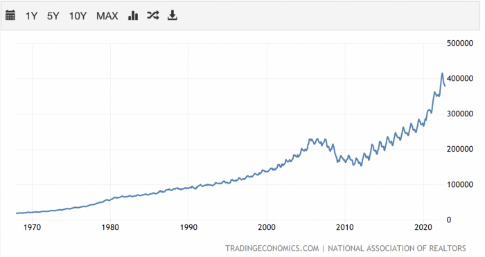
If you can buy a house, do it. You can refinance the interest at a lower rate with acceptable credit, but not the house price.
Take advantage of the housing market prices now because you won't find a decent deal when rates normalize.
How to profit from the cryptocurrency market.
This is the riskiest market to tackle right now, but it could offer the most opportunities if done appropriately.
The most powerful cryptocurrencies are down more than 60% from last year: $68,990 for BTC and $4,865 for ETH.
If you focus on those two coins, you can make 30%-60% without waiting for them to return to their ATH, and they're low enough to be a solid investment.
I don't encourage trying other altcoins because the crypto market is in crisis and you can lose everything if you're greedy.
Still, the main Cryptos are a good investment provided you store them in an external wallet and follow financial gurus' security advice.
Last thoughts
We can't anticipate a recession until it ends. We can't forecast a market or asset's lowest point, therefore waiting makes little sense.
If you want to develop your wealth, assess the money prospects on all the marketplaces and initiate long-term trades.
Many millionaires are made during recessions because they don't fear negative figures and use them to scale their money.
You might also like
Jumanne Rajabu Mtambalike
3 years ago
10 Years of Trying to Manage Time and Improve My Productivity.
I've spent the last 10 years of my career mastering time management. I've tried different approaches and followed multiple people and sources. My knowledge is summarized.
Great people, including entrepreneurs, master time management. I learned time management in college. I was studying Computer Science and Finance and leading Tanzanian students in Bangalore, India. I had 24 hours per day to do this and enjoy campus. I graduated and received several awards. I've learned to maximize my time. These tips and tools help me finish quickly.
Eisenhower-Box
I don't remember when I read the article. James Clear, one of my favorite bloggers, introduced me to the Eisenhower Box, which I've used for years. Eliminate waste to master time management. By grouping your activities by importance and urgency, the tool helps you prioritize what matters and drop what doesn't. If it's urgent, do it. Delegate if it's urgent but not necessary. If it's important but not urgent, reschedule it; otherwise, drop it. I integrated the tool with Trello to manage my daily tasks. Since 2007, I've done this.
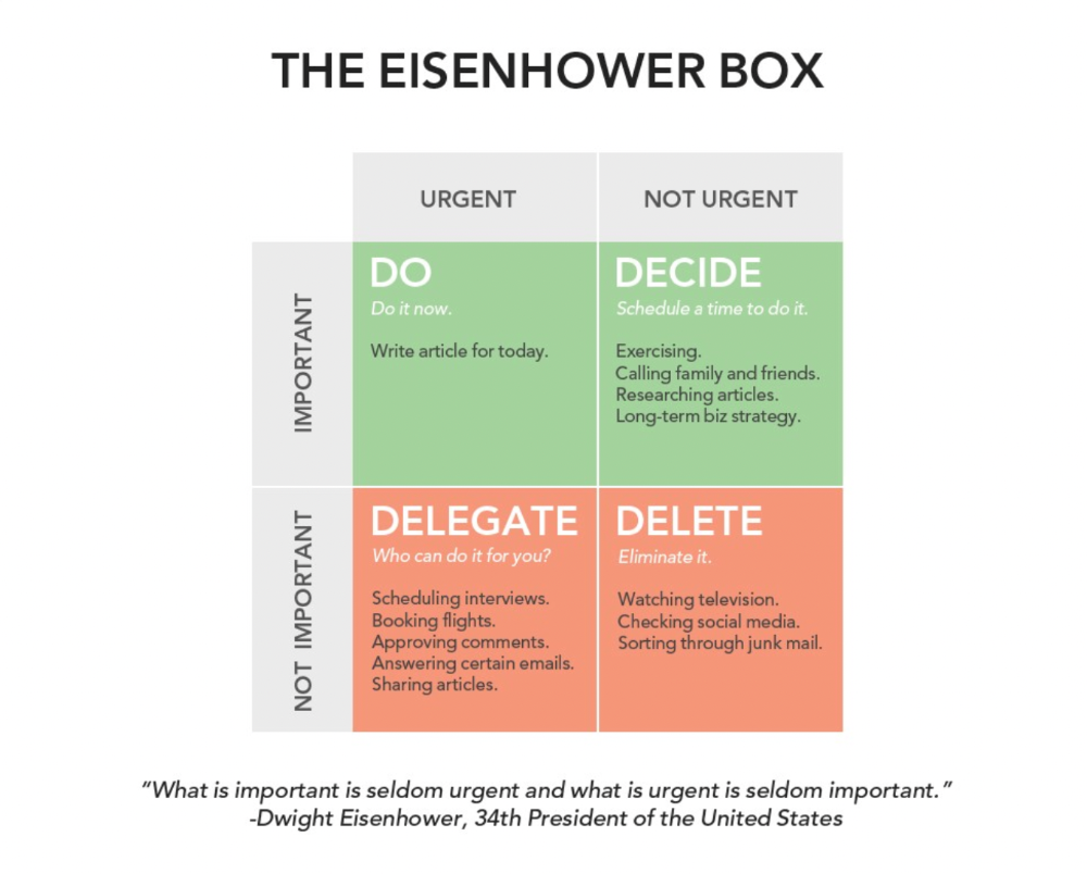
James Clear's article mentions Eisenhower Box.
Essentialism rules
Greg McKeown's book Essentialism introduced me to disciplined pursuit of less. I once wrote about this. I wasn't sure what my career's real opportunities and distractions were. A non-essentialist thinks everything is essential; you want to be everything to everyone, and your life lacks satisfaction. Poor time management starts it all. Reading and applying this book will change your life.
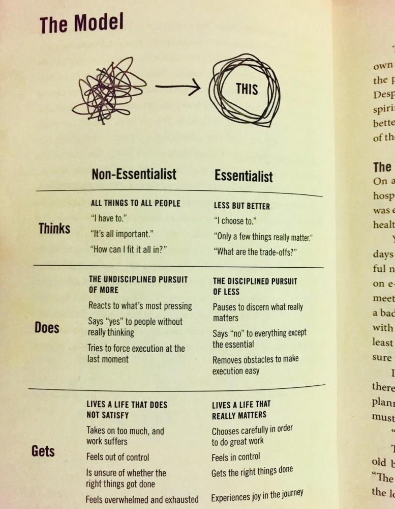
Essential vs non-essential
Life Calendar
Most of us make corporate calendars. Peter Njonjo, founder of Twiga Foods, said he manages time by putting life activities in his core calendars. It includes family retreats, weddings, and other events. He joked that his wife always complained to him to avoid becoming a calendar item. It's key. "Time Masters" manages life's four burners, not just work and corporate life. There's no "work-life balance"; it's life.
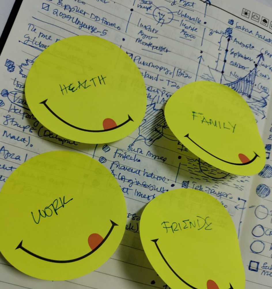
Health, Family, Work, and Friends.
The Brutal No
In a culture where people want to look good, saying "NO" to a favor request seems rude. In reality, the crime is breaking a promise. "Time Masters" have mastered "NO". More "YES" means less time, and more "NO" means more time for tasks and priorities. Brutal No doesn't mean being mean to your coworkers; it means explaining kindly and professionally that you have other priorities.
To-Do vs. MITs
Most people are productive with a routine to-do list. You can't be effective by just checking boxes on a To-do list. When was the last time you completed all of your daily tasks? Never. You must replace the to-do list with Most Important Tasks (MITs). MITs allow you to focus on the most important tasks on your list. You feel progress and accomplishment when you finish these tasks. MITs don't include ad-hoc emails, meetings, etc.
Journal Mapped
Most people don't journal or plan their day in the developing South. I've learned to plan my day in my journal over time. I have multiple sections on one page: MITs (things I want to accomplish that day), Other Activities (stuff I can postpone), Life (health, faith, and family issues), and Pop-Ups (things that just pop up). I leave the next page blank for notes. I reflected on the blocks to identify areas to improve the next day. You will have bad days, but at least you'll realize it was due to poor time management.
Buy time/delegate
Time or money? When you make enough money, you lose time to make more. The smart buy "Time." I resisted buying other people's time for years. I regret not hiring an assistant sooner. Learn to buy time from others and pay for time-consuming tasks. Sometimes you think you're saving money by doing things yourself, but you're actually losing money.
This post is a summary. See the full post here.

Chris Newman
3 years ago
Clean Food: Get Over Yourself If You Want to Save the World.

I’m a permaculture farmer. I want to create food-producing ecosystems. My hope is a world with easy access to a cuisine that nourishes consumers, supports producers, and leaves the Earth joyously habitable.
Permaculturists, natural farmers, plantsmen, and foodies share this ambition. I believe this group of green thumbs, stock-folk, and food champions is falling to tribalism, forgetting that rescuing the globe requires saving all of its inhabitants, even those who adore cheap burgers and Coke. We're digging foxholes and turning folks who disagree with us or don't understand into monsters.
Take Dr. Daphne Miller's comments at the end of her Slow Money Journal interview:
“Americans are going to fall into two camps when all is said and done: People who buy cheap goods, regardless of quality, versus people who are willing and able to pay for things that are made with integrity. We are seeing the limits of the “buying cheap crap” approach.”
This is one of the most judgmental things I've read outside the Bible. Consequences:
People who purchase inexpensive things (food) are ignorant buffoons who prefer to choose fair trade coffee over fuel as long as the price is correct.
It all depends on your WILL to buy quality or cheaply. Both those who are WILLING and those who ARE NOT exist. And able, too.
People who are unwilling and unable are purchasing garbage. You're giving your kids bad food. Both the Earth and you are being destroyed by your actions. Your camp is the wrong one. You’re garbage! Disgrace to you.
Dr. Miller didn't say it, but words are worthless until interpreted. This interpretation depends on the interpreter's economic, racial, political, religious, family, and personal history. Complementary language insults another. Imagine how that Brown/Harvard M.D.'s comment sounds to a low-income household with no savings.
Dr. Miller's comment reflects the echo chamber into which nearly all clean food advocates speak. It asks easy questions and accepts non-solutions like raising food prices and eating less meat. People like me have cultivated an insular world unencumbered by challenges beyond the margins. We may disagree about technical details in rotationally-grazing livestock, but we short circuit when asked how our system could supply half the global beef demand. Most people have never seriously considered this question. We're so loved and affirmed that challenging ourselves doesn't seem necessary. Were generals insisting we don't need to study the terrain because God is on our side?
“Yes, the $8/lb ground beef is produced the way it should be. Yes, it’s good for my body. Yes it’s good for the Earth. But it’s eight freaking dollars, and my kid needs braces and protein. Bye Felicia, we’re going to McDonald’s.”
-Bobby Q. Homemaker
Funny clean foodies. People don't pay enough for food; they should value it more. Turn the concept of buying food with integrity into a wedge and drive it into the heart of America, dividing the willing and unwilling.
We go apeshit if you call our products high-end.
I've heard all sorts of gaslighting to defend a $10/lb pork chop as accessible (things I’ve definitely said in the past):
At Whole Foods, it costs more.
The steak at the supermarket is overly affordable.
Pay me immediately or the doctor gets paid later.
I spoke with Timbercreek Market and Local Food Hub in front of 60 people. We were asked about local food availability.
They came to me last, after my co-panelists gave the same responses I would have given two years before.
I grumbled, "Our food is inaccessible." Nope. It's beyond the wallets of nearly everyone, and it's the biggest problem with sustainable food systems. We're criminally unserious about being leaders in sustainability until we propose solutions beyond economic relativism, wishful thinking, and insisting that vulnerable, distracted people do all the heavy lifting of finding a way to afford our food. And until we talk about solutions, all this preserve the world? False.
The room fell silent as if I'd revealed a terrible secret. Long, thunderous applause followed my other remarks. But I’m probably not getting invited back to any VNRLI events.
I make pricey cuisine. It’s high-end. I have customers who really have to stretch to get it, and they let me know it. They're forgoing other creature comforts to help me make a living and keep the Earth of my grandmothers alive, and they're doing it as an act of love. They believe in us and our work.
I remember it when I'm up to my shoulders in frigid water, when my vehicle stinks of four types of shit, when I come home covered in blood and mud, when I'm hauling water in 100-degree heat, when I'm herding pigs in a rainstorm and dodging lightning bolts to close the chickens. I'm reminded I'm not alone. Their enthusiasm is worth more than money; it helps me make a life and a living. I won't label that gift less than it is to make my meal seem more accessible.
Not everyone can sacrifice.
Let's not pretend we want to go back to peasant fare, despite our nostalgia. Industrial food has leveled what rich and poor eat. How food is cooked will be the largest difference between what you and a billionaire eat. Rich and poor have access to chicken, pork, and beef. You might be shocked how recently that wasn't the case. This abundance, particularly of animal protein, has helped vulnerable individuals.

Industrial food causes environmental damage, chronic disease, and distribution inequities. Clean food promotes non-industrial, artisan farming. This creates a higher-quality, more expensive product than the competition; we respond with aggressive marketing and the "people need to value food more" shtick geared at consumers who can spend the extra money.
The guy who is NOT able is rendered invisible by clean food's elitist marketing, which is bizarre given a.) clean food insists it's trying to save the world, yet b.) MOST PEOPLE IN THE WORLD ARE THAT GUY. No one can help him except feel-good charities. That's crazy.
Also wrong: a foodie telling a kid he can't eat a 99-cent fast food hamburger because it lacks integrity. Telling him how easy it is to save his ducketts and maybe have a grass-fed house burger at the end of the month as a reward, but in the meantime get your protein from canned beans you can't bake because you don't have a stove and, even if you did, your mom works two jobs and moonlights as an Uber driver so she doesn't have time to heat that shitup anyway.
A wealthy person's attitude toward the poor is indecent. It's 18th-century Versailles.

Human rights include access to nutritious food without social or environmental costs. As a food-forest-loving permaculture farmer, I no longer balk at the concept of cultured beef and hydroponics. My food is out of reach for many people, but access to decent food shouldn't be. Cultures and hydroponics could scale to meet the clean food affordability gap without externalities. If technology can deliver great, affordable beef without environmental negative effects, I can't reject it because it's new, unusual, or might endanger my business.
Why is your farm needed if cultured beef and hydroponics can feed the world? Permaculture food forests with trees, perennial plants, and animals are crucial to economically successful environmental protection. No matter how advanced technology gets, we still need clean air, water, soil, greenspace, and food.
Clean Food cultivated in/on live soil, minimally processed, and eaten close to harvest is part of the answer, not THE solution. Clean food advocates must recognize the conflicts at the intersection of environmental, social, and economic sustainability, the disproportionate effects of those conflicts on the poor and lower-middle classes, and the immorality and impracticality of insisting vulnerable people address those conflicts on their own and judging them if they don't.
Our clients, relatives, friends, and communities need an honest assessment of our role in a sustainable future. If we're serious about preserving the world, we owe honesty to non-customers. We owe our goal and sanity to honesty. Future health and happiness of the world left to the average person's pocketbook and long-term moral considerations is a dismal proposition with few parallels.
Let's make soil and grow food. Let the lab folks do their thing. We're all interdependent.

Hasan AboulHasan
3 years ago
High attachment products can help you earn money automatically.
Affiliate marketing is a popular online moneymaker. You promote others' products and get commissions. Affiliate marketing requires constant product promotion.
Affiliate marketing can be profitable even without much promotion. Yes, this is Autopilot Money.
How to Pick an Affiliate Program to Generate Income Autonomously
Autopilot moneymaking requires a recurring affiliate marketing program.
Finding the best product and testing it takes a lot of time and effort.
Here are three ways to choose the best service or product to promote:
Find a good attachment-rate product or service.
When choosing a product, ask if you can easily switch to another service. Attachment rate is how much people like a product.
Higher attachment rates mean better Autopilot products.
Consider promoting GetResponse. It's a 33% recurring commission email marketing tool. This means you get 33% of the customer's plan as long as he pays.
GetResponse has a high attachment rate because it's hard to leave and start over with another tool.
2. Pick a good or service with a lot of affiliate assets.
Check if a program has affiliate assets or creatives before joining.
Images and banners to promote the product in your business.
They save time; I look for promotional creatives. Creatives or affiliate assets are website banners or images. This reduces design time.
3. Select a service or item that consumers already adore.
New products are hard to sell. Choosing a trusted company's popular product or service is helpful.
As a beginner, let people buy a product they already love.
Online entrepreneurs and digital marketers love Systeme.io. It offers tools for creating pages, email marketing, funnels, and more. This product guarantees a high ROI.
Make the product known!
Affiliate marketers struggle to get traffic. Using affiliate marketing to make money is easier than you think if you have a solid marketing strategy.
Your plan should include:
1- Publish affiliate-related blog posts and SEO-optimize them
2- Sending new visitors product-related emails
3- Create a product resource page.
4-Review products
5-Make YouTube videos with links in the description.
6- Answering FAQs about your products and services on your blog and Quora.
7- Create an eCourse on how to use this product.
8- Adding Affiliate Banners to Your Website.
With these tips, you can promote your products and make money on autopilot.