(The author's opinions should not be used to make investment decisions or as a recommendation to invest.)

The pandemic and social media pseudoscience have made us all epidemiologists, for better or worse. Flattening the curve, social distancing, lockdowns—remember? Some of you may remember R0 (R naught), the number of healthy humans the average COVID-infected person infects. Thankfully, the world has moved on from Greater China's nightmare. Politicians have refocused their talent for misdirection on getting their constituents invested in the war for Russian Reunification or Russian Aggression, depending on your side of the iron curtain.

Humanity battles two fronts. A war against an invisible virus (I know your Commander in Chief might have told you COVID is over, but viruses don't follow election cycles and their economic impacts linger long after the last rapid-test clinic has closed); and an undeclared World War between US/NATO and Eurasia/Russia/China. The fiscal and monetary authorities' current policies aim to mitigate these two conflicts' economic effects.

Since all politicians are short-sighted, they usually print money to solve most problems. Printing money is the easiest and fastest way to solve most problems because it can be done immediately without much discussion. The alternative—long-term restructuring of our global economy—would hurt stakeholders and require an honest discussion about our civilization's state. Both of those requirements are non-starters for our short-sighted political friends, so whether your government practices capitalism, communism, socialism, or fascism, they all turn to printing money-ism to solve all problems.

Free money stimulates demand, so people buy crap. Overbuying shit raises prices. Inflation. Every nation has food, energy, or goods inflation. The once-docile plebes demand action when the latter two subsets of inflation rise rapidly. They will be heard at the polls or in the streets. What would you do to feed your crying hungry child?

Global central banks During the pandemic, the Fed, PBOC, BOJ, ECB, and BOE printed money to aid their governments. They worried about inflation and promised to remove fiat liquidity and tighten monetary conditions.

Imagine Nate Diaz's round-house kick to the face. The financial markets probably felt that way when the US and a few others withdrew fiat wampum. Sovereign debt markets suffered a near-record bond market rout.

The undeclared WW3 is intensifying, with recent gas pipeline attacks. The global economy is already struggling, and credit withdrawal will worsen the situation. The next pandemic, the Yield Curve Control (YCC) virus, is spreading as major central banks backtrack on inflation promises. All central banks eventually fail.

Here's a scorecard.

In order to save its financial system, BOE recently reverted to Quantitative Easing (QE).

BOJ Continuing YCC to save their banking system and enable affordable government borrowing.

ECB printing money to buy weak EU member bonds, but will soon start Quantitative Tightening (QT).

PBOC Restarting the money printer to give banks liquidity to support the falling residential property market.

Fed raising rates and QT-shrinking balance sheet.

80% of the world's biggest central banks are printing money again. Only the Fed has remained steadfast in the face of a financial market bloodbath, determined to end the inflation for which it is at least partially responsible—the culmination of decades of bad economic policies and a world war.

YCC printing is the worst for fiat currency and society. Because it necessitates central banks fixing a multi-trillion-dollar bond market. YCC central banks promise to infinitely expand their balance sheets to keep a certain interest rate metric below an unnatural ceiling. The market always wins, crushing humanity with inflation.

BOJ's YCC policy is longest-standing. The BOE joined them, and my essay this week argues that the ECB will follow. The ECB joining YCC would make 60% of major central banks follow this terrible policy. Since the PBOC is part of the Chinese financial system, the number could be 80%. The Chinese will lend any amount to meet their economic activity goals.

The BOE committed to a 13-week, GBP 65bn bond price-fixing operation. However, BOEs YCC may return. If you lose to the market, you're stuck. Since the BOE has announced that it will buy your Gilt at inflated prices, why would you not sell them all? Market participants taking advantage of this policy will only push the bank further into the hole it dug itself, so I expect the BOE to re-up this program and count them as YCC.

In a few trading days, the BOE went from a bank determined to slay inflation by raising interest rates and QT to buying an unlimited amount of UK Gilts. I expect the ECB to be dragged kicking and screaming into a similar policy. Spoiler alert: big daddy Fed will eventually die from the YCC virus.

Threadneedle St, London EC2R 8AH, UK

Before we discuss the BOE's recent missteps, a chatroom member called the British royal family the Kardashians with Crowns, which made me laugh. I'm sad about royal attention. If the public was as interested in energy and economic policies as they are in how the late Queen treated Meghan, Duchess of Sussex, UK politicians might not have been able to get away with energy and economic fairy tales.

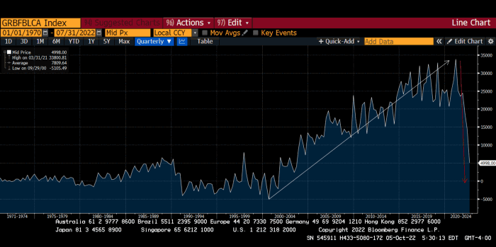
The BOE printed money to recover from COVID, as all good central banks do. For historical context, this chart shows the BOE's total assets as a percentage of GDP since its founding in the 18th century.

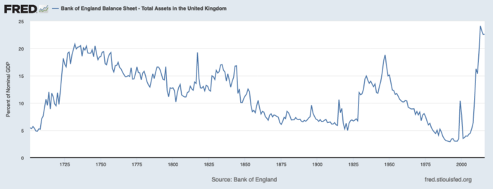
The UK has had a rough three centuries. Pandemics, empire wars, civil wars, world wars. Even so, the BOE's recent money printing was its most aggressive ever!

BOE Total Assets as % of GDP (white) vs. UK CPI

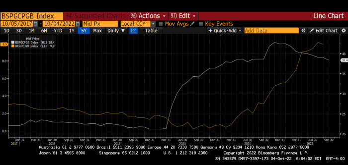
Now, inflation responded slowly to the bank's most aggressive monetary loosening. King Charles wishes the gold line above showed his popularity, but it shows his subjects' suffering.

The BOE recognized early that its money printing caused runaway inflation. In its August 2022 report, the bank predicted that inflation would reach 13% by year end before aggressively tapering in 2023 and 2024.

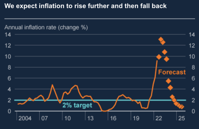
Aug 2022 BOE Monetary Policy Report

The BOE was the first major central bank to reduce its balance sheet and raise its policy rate to help.

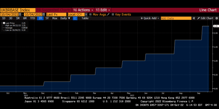
The BOE first raised rates in December 2021. Back then, JayPow wasn't even considering raising rates.

UK policymakers, like most developed nations, believe in energy fairy tales. Namely, that the developed world, which grew in lockstep with hydrocarbon use, could switch to wind and solar by 2050. The UK's energy import bill has grown while coal, North Sea oil, and possibly stranded shale oil have been ignored.

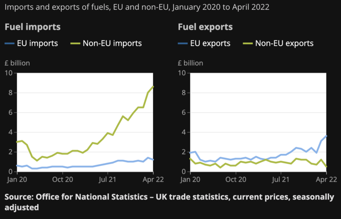
WW3 is an economic war that is balkanizing energy markets, which will continue to inflate. A nation that imports energy and has printed the most money in its history cannot avoid inflation.

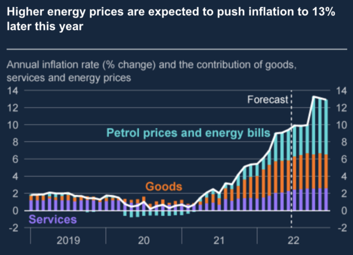
The chart above shows that energy inflation is a major cause of plebe pain.

The UK is hit by a double whammy: the BOE must remove credit to reduce demand, and energy prices must rise due to WW3 inflation. That's not economic growth.

Boris Johnson was knocked out by his country's poor economic performance, not his lockdown at 10 Downing St. Prime Minister Truss and her merry band of fools arrived with the tried-and-true government remedy: goodies for everyone.

She released a budget full of economic stimulants. She cut corporate and individual taxes for the rich. She plans to give poor people vouchers for higher energy bills. Woohoo! Margret Thatcher's new pants suit.

My buddy Jim Bianco said Truss budget's problem is that it works. It will boost activity at a time when inflation is over 10%. Truss' budget didn't include austerity measures like tax increases or spending cuts, which the bond market wanted. The bond market protested.

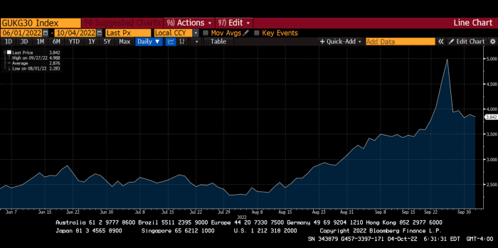
30-year Gilt yield chart. Yields spiked the most ever after Truss announced her budget, as shown. The Gilt market is the longest-running bond market in the world.

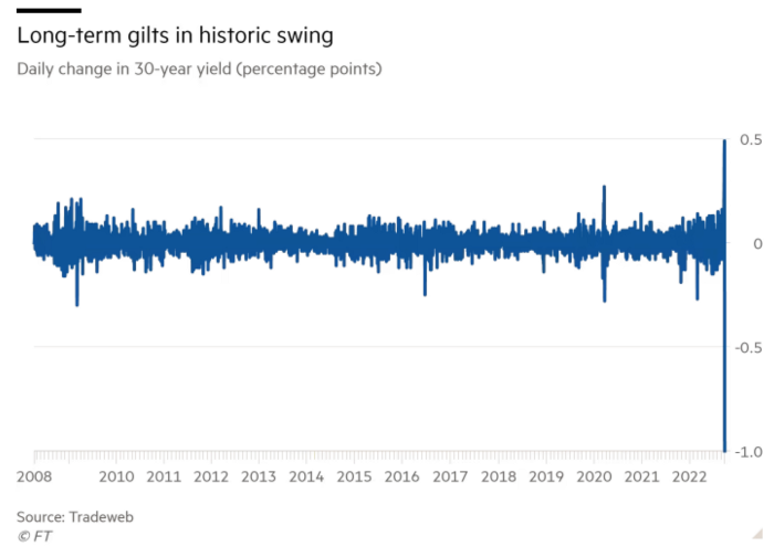
The Gilt market showed the pole who's boss with Cardi B.

Before this, the BOE was super-committed to fighting inflation. To their credit, they raised short-term rates and shrank their balance sheet. However, rapid yield rises threatened to destroy the entire highly leveraged UK financial system overnight, forcing them to change course.

Accounting gimmicks allowed by regulators for pension funds posed a systemic threat to the UK banking system. UK pension funds could use interest rate market levered derivatives to match liabilities. When rates rise, short rate derivatives require more margin. The pension funds spent all their money trying to pick stonks and whatever else their sell side banker could stuff them with, so the historic rate spike would have bankrupted them overnight. The FT describes BOE-supervised chicanery well.

To avoid a financial apocalypse, the BOE in one morning abandoned all their hard work and started buying unlimited long-dated Gilts to drive prices down.

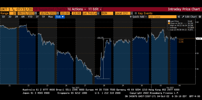
Another reminder to never fight a central bank. The 30-year Gilt is shown above. After the BOE restarted the money printer on September 28, this bond rose 30%. Thirty-fucking-percent! Developed market sovereign bonds rarely move daily. You're invested in His Majesty's government obligations, not a Chinese property developer's offshore USD bond.

The political need to give people goodies to help them fight the terrible economy ran into a financial reality. The central bank protected the UK financial system from asset-price deflation because, like all modern economies, it is debt-based and highly levered. As bad as it is, inflation is not their top priority. The BOE example demonstrated that. To save the financial system, they abandoned almost a year of prudent monetary policy in a few hours. They also started the endgame.

Let's play Central Bankers Say the Darndest Things before we go to the continent (and sorry if you live on a continent other than Europe, but you're not culturally relevant).

Pre-meltdown BOE output:

FT, October 17, 2021 On Sunday, the Bank of England governor warned that it must act to curb inflationary pressure, ignoring financial market moves that have priced in the first interest rate increase before the end of the year.

On July 19, 2022, Gov. Andrew Bailey spoke. Our 2% inflation target is unwavering. We'll do our job.

August 4th 2022 MPC monetary policy announcement According to its mandate, the MPC will sustainably return inflation to 2% in the medium term.

Catherine Mann, MPC member, September 5, 2022 speech. Fast and forceful monetary tightening, possibly followed by a hold or reversal, is better than gradualism because it promotes inflation expectations' role in bringing inflation back to 2% over the medium term.

When their financial system nearly collapsed in one trading session, they said:

The Bank of England's Financial Policy Committee warned on 28 September that gilt market dysfunction threatened UK financial stability. It advised action and supported the Bank's urgent gilt market purchases for financial stability.

It works when the price goes up but not down. Is my crypto portfolio dysfunctional enough to get a BOE bailout?

Next, the EU and ECB. The ECB is also fighting inflation, but it will also succumb to the YCC virus for the same reasons as the BOE.

Frankfurt am Main, ECB Tower, Sonnemannstraße 20, 60314

Only France and Germany matter economically in the EU. Modern European history has focused on keeping Germany and Russia apart. German manufacturing and cheap Russian goods could change geopolitics.

France created the EU to keep Germany down, and the Germans only cooperated because of WWII guilt. France's interests are shared by the US, which lurks in the shadows to prevent a Germany-Russia alliance. A weak EU benefits US politics. Avoid unification of Eurasia. (I paraphrased daddy Felix because I thought quoting a large part of his most recent missive would get me spanked.)

As with everything, understanding Germany's energy policy is the best way to understand why the German economy is fundamentally fucked and why that spells doom for the EU. Germany, the EU's main economic engine, is being crippled by high energy prices, threatening a depression. This economic downturn threatens the union. The ECB may have to abandon plans to shrink its balance sheet and switch to YCC to save the EU's unholy political union.

France did the smart thing and went all in on nuclear energy, which is rare in geopolitics. 70% of electricity is nuclear-powered. Their manufacturing base can survive Russian gas cuts. Germany cannot.

My boy Zoltan made this great graphic showing how screwed Germany is as cheap Russian gas leaves the industrial economy.

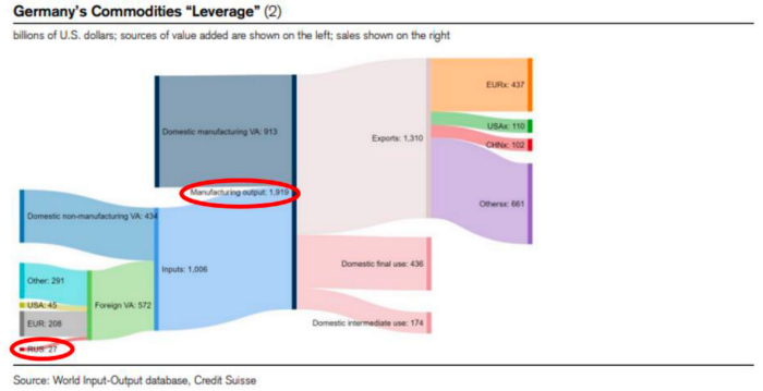
$27 billion of Russian gas powers almost $2 trillion of German economic output, a 75x energy leverage. The German public was duped into believing the same energy fairy tales as their politicians, and they overwhelmingly allowed the Green party to dismantle any efforts to build a nuclear energy ecosystem over the past several decades. Germany, unlike France, must import expensive American and Qatari LNG via supertankers due to Nordstream I and II pipeline sabotage.

American gas exports to Europe are touted by the media. Gas is cheap because America isn't the Western world's swing producer. If gas prices rise domestically in America, the plebes would demand the end of imports to avoid paying more to heat their homes.

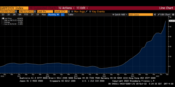
German goods would cost much more in this scenario. German producer prices rose 46% YoY in August. The German current account is rapidly approaching zero and will soon be negative.

German PPI Change YoY

German Current Account

The reason this matters is a curious construction called TARGET2. Let’s hear from the horse’s mouth what exactly this beat is:

TARGET2 is the real-time gross settlement (RTGS) system owned and operated by the Eurosystem. Central banks and commercial banks can submit payment orders in euro to TARGET2, where they are processed and settled in central bank money, i.e. money held in an account with a central bank.

Source: ECB

Let me explain this in plain English for those unfamiliar with economic dogma.

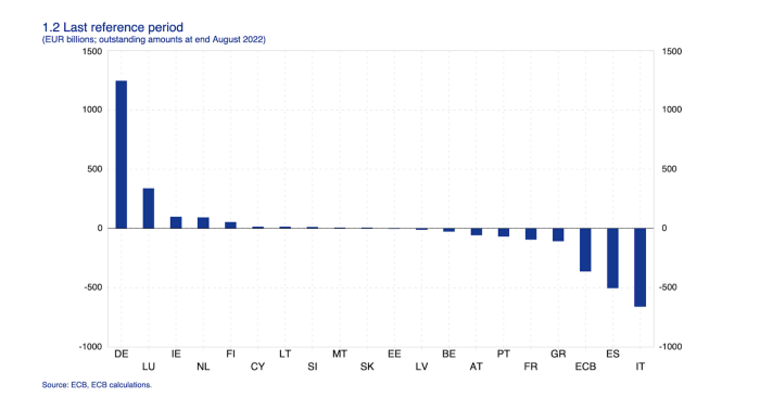
This chart shows intra-EU credits and debits. TARGET2. Germany, Europe's powerhouse, is owed money. IOU-buying Greeks buy G-wagons. The G-wagon pickup truck is badass.

If all EU countries had fiat currencies, the Deutsche Mark would be stronger than the Italian Lira, according to the chart above. If Europe had to buy goods from non-EU countries, the Euro would be much weaker. Credits and debits between smaller political units smooth out imbalances in other federal-provincial-state political systems. Financial and fiscal unions allow this. The EU is financial, so the centre cannot force the periphery to settle their imbalances.

Greece has never had to buy Fords or Kias instead of BMWs, but what if Germany had to shut down its auto manufacturing plants due to energy shortages?

Italians have done well buying ammonia from Germany rather than China, but what if BASF had to close its Ludwigshafen facility due to a lack of affordable natural gas?

I think you're seeing the issue.

Instead of Germany, EU countries would owe foreign producers like America, China, South Korea, Japan, etc. Since these countries aren't tied into an uneconomic union for politics, they'll demand hard fiat currency like USD instead of Euros, which have become toilet paper (or toilet plastic).

Keynesian economists have a simple solution for politicians who can't afford market prices. Government debt can maintain production. The debt covers the difference between what a business can afford and the international energy market price.

Germans are monetary policy conservative because of the Weimar Republic's hyperinflation. The Bundesbank is the only thing preventing ECB profligacy. Germany must print its way out without cheap energy. Like other nations, they will issue more bonds for fiscal transfers.

More Bunds mean lower prices. Without German monetary discipline, the Euro would have become a trash currency like any other emerging market that imports energy and food and has uncompetitive labor.

Bunds price all EU country bonds. The ECB's money printing is designed to keep the spread of weak EU member bonds vs. Bunds low. Everyone falls with Bunds.

Like the UK, German politicians seeking re-election will likely cause a Bunds selloff. Bond investors will understandably reject their promises of goodies for industry and individuals to offset the lack of cheap Russian gas. Long-dated Bunds will be smoked like UK Gilts. The ECB will face a wave of ultra-levered financial players who will go bankrupt if they mark to market their fixed income derivatives books at higher Bund yields.

Some treats People: Germany will spend 200B to help consumers and businesses cope with energy prices, including promoting renewable energy.

That, ladies and germs, is why the ECB will immediately abandon QT, move to a stop-gap QE program to normalize the Bund and every other EU bond market, and eventually graduate to YCC as the market vomits bonds of all stripes into Christine Lagarde's loving hands. She probably has soft hands.

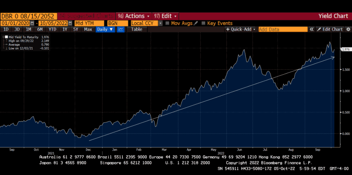
The 30-year Bund market has noticed Germany's economic collapse. 2021 yields skyrocketed.

30-year Bund Yield

ECB Says the Darndest Things:

Because inflation is too high and likely to stay above our target for a long time, we took today's decision and expect to raise interest rates further.- Christine Lagarde, ECB Press Conference, Sept 8.

The Governing Council will adjust all of its instruments to stabilize inflation at 2% over the medium term. July 21 ECB Monetary Decision

Everyone struggles with high inflation. The Governing Council will ensure medium-term inflation returns to two percent. June 9th ECB Press Conference

I'm excited to read the after. Like the BOE, the ECB may abandon their plans to shrink their balance sheet and resume QE due to debt market dysfunction.

Eighty Percent

I like YCC like dark chocolate over 80%. ;).

Can 80% of the world's major central banks' QE and/or YCC overcome Sir Powell's toughness on fungible risky asset prices?

Gold and crypto are fungible global risky assets. Satoshis and gold bars are the same in New York, London, Frankfurt, Tokyo, and Shanghai.

As more Euros, Yen, Renminbi, and Pounds are printed, people will move their savings into Dollars or other stores of value. As the Fed raises rates and reduces its balance sheet, the USD will strengthen. Gold/EUR and BTC/JPY may also attract buyers.

Gold and crypto markets are much smaller than the trillions in fiat money that will be printed, so they will appreciate in non-USD currencies. These flows only matter in one instance because we trade the global or USD price. Arbitrage occurs when BTC/EUR rises faster than EUR/USD. Here is how it works:

1. An investor based in the USD notices that BTC is expensive in EUR terms.

2. Instead of buying BTC, this investor borrows USD and then sells it.

3. After that, they sell BTC and buy EUR.

4. Then they choose to sell EUR and buy USD.

5. The investor receives their profit after repaying the USD loan.

This triangular FX arbitrage will align the global/USD BTC price with the elevated EUR, JPY, CNY, and GBP prices.

Even if the Fed continues QT, which I doubt they can do past early 2023, small stores of value like gold and Bitcoin may rise as non-Fed central banks get serious about printing money.

“Arthur, this is just more copium,” you might retort.

Patience. This takes time. Economic and political forcing functions take time. The BOE example shows that bond markets will reject politicians' policies to appease voters. Decades of bad energy policy have no immediate fix. Money printing is the only politically viable option. Bond yields will rise as bond markets see more stimulative budgets, and the over-leveraged fiat debt-based financial system will collapse quickly, followed by a monetary bailout.

America has enough food, fuel, and people. China, Europe, Japan, and the UK suffer. America can be autonomous. Thus, the Fed can prioritize domestic political inflation concerns over supplying the world (and most of its allies) with dollars. A steady flow of dollars allows other nations to print their currencies and buy energy in USD. If the strongest player wins, everyone else loses.

I'm making a GDP-weighted index of these five central banks' money printing. When ready, I'll share its rate of change. This will show when the 80%'s money printing exceeds the Fed's tightening.

Bear markets don't last forever, but that's hard to remember. Jamie Cullen's illustration

A bear market is a 20% decline from peak to trough in stock prices.

The S&P 500 was down 24% from its January highs at its low point this year. Bear market.

The U.S. stock market has had 13 bear markets since WWII (including the current one). Previous 12 bear markets averaged –32.7% losses. From peak to trough, the stock market averaged 12 months. The average time from bottom to peak was 21 months.

In the past seven decades, a bear market roundtrip to breakeven has averaged less than three years.

Long-term averages can vary widely, as with all historical market data. Investors can learn from past market crashes.

Historical bear markets offer lessons.

Bear market duration

A bear market can cost investors money and time. Most of the pain comes from stock market declines, but bear markets can be long.

Here are the longest U.S. stock bear markets since World war 2:

Stock market crashes can make it difficult to break even. After the 2008 financial crisis, the stock market took 4.5 years to recover. After the dotcom bubble burst, it took seven years to break even.

The longer you're underwater in the market, the more suffering you'll experience, according to research. Suffering can lead to selling at the wrong time.

Bear markets require patience because stocks can take a long time to recover.

Stock crash recovery

Bear markets can end quickly. The Corona Crash in early 2020 is an example.

The S&P 500 fell 34% in 23 trading sessions, the fastest bear market from a high in 90 years. The entire crash lasted one month. Stocks broke even six months after bottoming. Stocks rose 100% from those lows in 15 months.

Seven bear markets have lasted two years or less since 1945.

The 2020 recovery was an outlier, but four other bear markets have made investors whole within 18 months.

During a bear market, you don't know if it will end quickly or feel like death by a thousand cuts.

Recessions vs. bear markets

Many people believe the U.S. economy is in or heading for a recession.

I agree. Four-decade high inflation. Since 1945, inflation has exceeded 5% nine times. Each inflationary spike caused a recession. Only slowing economic demand seems to stop price spikes.

This could happen again. Stocks seem to be pricing in a recession.

Recessions almost always cause a bear market, but a bear market doesn't always equal a recession. In 1946, the stock market fell 27% without a recession in sight. Without an economic slowdown, the stock market fell 22% in 1966. Black Monday in 1987 was the most famous stock market crash without a recession. Stocks fell 30% in less than a week. Many believed the stock market signaled a depression. The crash caused no slowdown.

Economic cycles are hard to predict. Even Wall Street makes mistakes.

Bears vs. bulls

Bear markets for U.S. stocks always end. Every stock market crash in U.S. history has been followed by new all-time highs.

How should investors view the recession? Investing risk is subjective.

You don't have as long to wait out a bear market if you're retired or nearing retirement. Diversification and liquidity help investors with limited time or income. Cash and short-term bonds drag down long-term returns but can ensure short-term spending.

Young people with years or decades ahead of them should view this bear market as an opportunity. Stock market crashes are good for net savers in the future. They let you buy cheap stocks with high dividend yields.

You need discipline, patience, and planning to buy stocks when it doesn't feel right.

Bear markets aren't fun because no one likes seeing their portfolio fall. But stock market downturns are a feature, not a bug. If stocks never crashed, they wouldn't offer such great long-term returns.

Software can change any company.

Software is becoming essential. Everyone should consider how software affects their lives and others'.

Software on your phone, tablet, or computer offers many new options. We're experts in enough ways now.

Software Business Ideas will be popular by 2023.

ERP Programs

ERP software meets rising demand.

ERP solutions automate and monitor tasks that large organizations, businesses, and even schools would struggle to do manually.

ERP software could reach $49 billion by 2024.

CRM Program

CRM software is a must-have for any customer-focused business.

Having an open mind about your business services and products allows you to change platforms.

Another company may only want your CRM service.

Medical software

Healthcare facilities need reliable, easy-to-use software.

EHRs, MDDBs, E-Prescribing, and more are software options.

The global medical software market could reach $11 billion by 2025, and mobile medical apps may follow.

Presentation Software in the Cloud

SaaS presentation tools are great.

They're easy to use, comprehensive, and full of traditional Software features.

In today's cloud-based world, these solutions make life easier for people. We don't know about you, but we like it.

Software for Project Management

People began working remotely without signs or warnings before the 2020 COVID-19 pandemic.

Many organizations found it difficult to track projects and set deadlines.

With PMP software tools, teams can manage remote units and collaborate effectively.

App for Blockchain-Based Invoicing

This advanced billing and invoicing solution is for businesses and freelancers.

These blockchain-based apps can calculate taxes, manage debts, and manage transactions.

Intelligent contracts help blockchain track transactions more efficiently. It speeds up and improves invoice generation.

Software for Business Communications

Internal business messaging is tricky.

Top business software tools for communication can share files, collaborate on documents, host video conferences, and more.

Payroll Automation System

Software development also includes developing an automated payroll system.

These software systems reduce manual tasks for timely employee payments.

These tools help enterprise clients calculate total wages quickly, simplify tax calculations, improve record-keeping, and support better financial planning.

System for Detecting Data Leaks

Both businesses and individuals value data highly. Yahoo's data breach is dangerous because of this.

This area of software development can help people protect their data.

You can design an advanced data loss prevention system.

AI-based Retail System

AI-powered shopping systems are popular. The systems analyze customers' search and purchase patterns and store history and are equipped with a keyword database.

These systems offer many customers pre-loaded products.

AI-based shopping algorithms also help users make purchases.

Software for Detecting Plagiarism

Software can help ensure your projects are original and not plagiarized.

These tools detect plagiarized content that Google, media, and educational institutions don't like.

Software for Converting Audio to Text

Machine Learning converts speech to text automatically.

These programs can quickly transcribe cloud-based files.

Software for daily horoscopes

Daily and monthly horoscopes will continue to be popular.

Software platforms that can predict forecasts, calculate birth charts, and other astrology resources are good business ideas.

E-learning Programs

Traditional study methods are losing popularity as virtual schools proliferate and physical space shrinks.

Khan Academy online courses are the best way to keep learning.

Online education portals can boost your learning. If you want to start a tech startup, consider creating an e-learning program.

Conclusion

Software is booming. There's never been a better time to start a software development business, with so many people using computers and smartphones. This article lists eight business ideas for 2023. Consider these ideas if you're just starting out or looking to expand.

Smarter work yields better results.

17-year-old me worked and studied 20 hours a day. During school breaks, I did coursework and ran a nonprofit at night. Long hours earned me national campaigns, A-list opportunities, and a great career. As I aged, my thoughts changed. Working harder isn't necessarily the key to success.

In some cases, doing less work might lead to better outcomes.

Consider a hard-working small business owner. He can't beat his corporate rivals by working hard. Time's limited. An entrepreneur can work 24 hours a day, 7 days a week, but a rival can invest more money, create a staff, and put in more man hours. Why have small startups done what larger companies couldn't? Facebook paid $1 billion for 13-person Instagram. Snapchat, a 30-person startup, rejected Facebook and Google bids. Luck and efficiency each contributed to their achievement.

The key to success is not working hard. It’s working smart.

Being busy and productive are different. Busy doesn't always equal productive. Productivity is less about time management and more about energy management. Life's work. It's using less energy to obtain more rewards. I cut my work week from 80 to 40 hours and got more done. I value simplicity.

Here are seven activities I gave up in order to be more productive.

1. Give up working extra hours and boost productivity instead.

When did the five-day, 40-hour work week start? Henry Ford, Ford Motor Company founder, experimented with his workers in 1926.

He decreased their daily hours from 10 to 8, and shortened the work week from 6 days to 5. As a result, he saw his workers’ productivity increase.

According to a 1980 Business Roundtable report, Scheduled Overtime Effect on Construction Projects, the more you work, the less effective and productive you become.

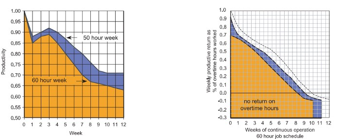
“Where a work schedule of 60 or more hours per week is continued longer than about two months, the cumulative effect of decreased productivity will cause a delay in the completion date beyond that which could have been realized with the same crew size on a 40-hour week.” Source: Calculating Loss of Productivity Due to Overtime Using Published Charts — Fact or Fiction

AlterNet editor Sara Robinson cited US military research showing that losing one hour of sleep per night for a week causes cognitive impairment equivalent to a.10 blood alcohol level. You can get fired for showing up drunk, but an all-nighter is fine.

Irrespective of how well you were able to get on with your day after that most recent night without sleep, it is unlikely that you felt especially upbeat and joyous about the world. Your more-negative-than-usual perspective will have resulted from a generalized low mood, which is a normal consequence of being overtired. More important than just the mood, this mind-set is often accompanied by decreases in willingness to think and act proactively, control impulses, feel positive about yourself, empathize with others, and generally use emotional intelligence. Source: The Secret World of Sleep: The Surprising Science of the Mind at Rest

To be productive, don't overwork and get enough sleep. If you're not productive, lack of sleep may be to blame. James Maas, a sleep researcher and expert, said 7/10 Americans don't get enough sleep.

Did you know?

• Leonardo da Vinci slept little at night and frequently took naps.

• Napoleon, the French emperor, had no qualms about napping. He splurged every day.

• Even though Thomas Edison felt self-conscious about his napping behavior, he regularly engaged in this ritual.

• President Franklin D. Roosevelt's wife Eleanor used to take naps before speeches to increase her energy.

• The Singing Cowboy, Gene Autry, was known for taking regular naps in his dressing area in between shows.

• Every day, President John F. Kennedy took a siesta after eating his lunch in bed.

• Every afternoon, oil businessman and philanthropist John D. Rockefeller took a nap in his office.

• It was unavoidable for Winston Churchill to take an afternoon snooze. He thought it enabled him to accomplish twice as much each day.

• Every afternoon around 3:30, President Lyndon B. Johnson took a nap to divide his day into two segments.

• Ronald Reagan, the 40th president, was well known for taking naps as well.

Source: 5 Reasons Why You Should Take a Nap Every Day — Michael Hyatt

Since I started getting 7 to 8 hours of sleep a night, I've been more productive and completed more work than when I worked 16 hours a day. Who knew marketers could use sleep?

2. Refrain from accepting too frequently

Pareto's principle states that 20% of effort produces 80% of results, but 20% of results takes 80% of effort. Instead of working harder, we should prioritize the initiatives that produce the most outcomes. So we can focus on crucial tasks. Stop accepting unproductive tasks.

“The difference between successful people and very successful people is that very successful people say “no” to almost everything.” — Warren Buffett

What should you accept? Why say no? Consider doing a split test to determine if anything is worth your attention. Track what you do, how long it takes, and the consequences. Then, evaluate your list to discover what worked (or didn't) to optimize future chores.

Most of us say yes more often than we should, out of guilt, overextension, and because it's simpler than no. Nobody likes being awful.

Researchers separated 120 students into two groups for a 2012 Journal of Consumer Research study. One group was educated to say “I can't” while discussing choices, while the other used “I don't”.

The students who told themselves “I can’t eat X” chose to eat the chocolate candy bar 61% of the time. Meanwhile, the students who told themselves “I don’t eat X” chose to eat the chocolate candy bars only 36% of the time. This simple change in terminology significantly improved the odds that each person would make a more healthy food choice.

Next time you need to say no, utilize I don't to encourage saying no to unimportant things.

The 20-second rule is another wonderful way to avoid pursuits with little value. Add a 20-second roadblock to things you shouldn't do or bad habits you want to break. Delete social media apps from your phone so it takes you 20 seconds to find your laptop to access them. You'll be less likely to engage in a draining hobby or habit if you add an inconvenience.

Lower the activation energy for habits you want to adopt and raise it for habits you want to avoid. The more we can lower or even eliminate the activation energy for our desired actions, the more we enhance our ability to jump-start positive change. Source: The Happiness Advantage: The Seven Principles of Positive Psychology That Fuel Success and Performance at Work

3. Stop doing everything yourself and start letting people help you

I once managed a large community and couldn't do it alone. The community took over once I burned out. Members did better than I could have alone. I learned about community and user-generated content.

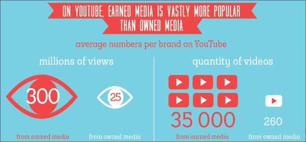
Consumers know what they want better than marketers. Octoly says user-generated videos on YouTube are viewed 10 times more than brand-generated videos. 51% of Americans trust user-generated material more than a brand's official website (16%) or media coverage (22%). (14 percent). Marketers should seek help from the brand community.

Being a successful content marketer isn't about generating the best content, but cultivating a wonderful community.

We should seek aid when needed. We can't do everything. It's best to delegate work so you may focus on the most critical things. Instead of overworking or doing things alone, let others help.

Having friends or coworkers around can boost your productivity even if they can't help.

Just having friends nearby can push you toward productivity. “There’s a concept in ADHD treatment called the ‘body double,’ ” says David Nowell, Ph.D., a clinical neuropsychologist from Worcester, Massachusetts. “Distractable people get more done when there is someone else there, even if he isn’t coaching or assisting them.” If you’re facing a task that is dull or difficult, such as cleaning out your closets or pulling together your receipts for tax time, get a friend to be your body double. Source: Friendfluence: The Surprising Ways Friends Make Us Who We Are

4. Give up striving for perfection

Perfectionism hinders professors' research output. Dr. Simon Sherry, a psychology professor at Dalhousie University, did a study on perfectionism and productivity. Dr. Sherry established a link between perfectionism and productivity.

Perfectionism has its drawbacks.

• They work on a task longer than necessary.

• They delay and wait for the ideal opportunity. If the time is right in business, you are already past the point.

• They pay too much attention to the details and miss the big picture.

Marketers await the right time. They miss out.

The perfect moment is NOW.

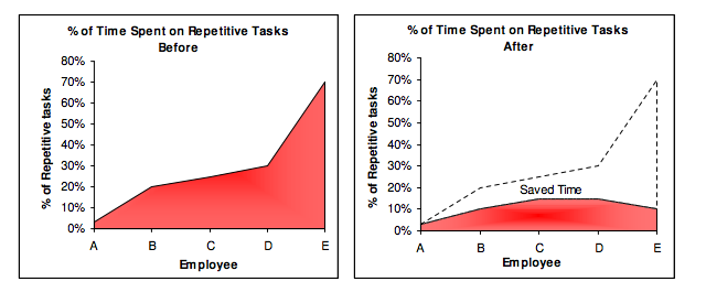
5. Automate monotonous chores instead of continuing to do them.

A team of five workers who spent 3%, 20%, 25%, 30%, and 70% of their time on repetitive tasks reduced their time spent to 3%, 10%, 15%, 15%, and 10% after two months of working to improve their productivity.

Last week, I wrote a 15-minute Python program. I wanted to generate content utilizing Twitter API data and Hootsuite to bulk schedule it. Automation has cut this task from a day to five minutes. Whenever I do something more than five times, I try to automate it.

Automate monotonous chores without coding. Skills and resources are nice, but not required.  If you cannot build it, buy it.

People forget time equals money. Manual work is easy and requires little investigation. You can moderate 30 Instagram photographs for your UGC campaign. You need digital asset management software to manage 30,000 photographs and movies from five platforms. Filemobile helps individuals develop more user-generated content. You may buy software to manage rich media and address most internet difficulties.

Hire an expert if you can't find a solution. Spend money to make money, and time is your most precious asset.

Visit GitHub or Google Apps Script library, marketers. You may often find free, easy-to-use open source code.

6. Stop relying on intuition and start supporting your choices with data.

You may optimize your life by optimizing webpages for search engines.

Numerous studies might help you boost your productivity. Did you know individuals are most distracted from midday to 4 p.m.? This is what a Penn State psychology professor found. Even if you can't find data on a particular question, it's easy to run a split test and review your own results.

7. Stop working and spend some time doing absolutely nothing.

Most people don't know that being too focused can be destructive to our work or achievements. The Boston Globe's The Power of Lonely says solo time is excellent for the brain and spirit.

One ongoing Harvard study indicates that people form more lasting and accurate memories if they believe they’re experiencing something alone. Another indicates that a certain amount of solitude can make a person more capable of empathy towards others. And while no one would dispute that too much isolation early in life can be unhealthy, a certain amount of solitude has been shown to help teenagers improve their moods and earn good grades in school. Source: The Power of Lonely

Reflection is vital. We find solutions when we're not looking.

We don't become more productive overnight. It demands effort and practice. Waiting for change doesn't work. Instead, learn about your body and identify ways to optimize your energy and time for a happy existence.