


More on Economics & Investing

Sofien Kaabar, CFA
2 years ago
Innovative Trading Methods: The Catapult Indicator
Python Volatility-Based Catapult Indicator
As a catapult, this technical indicator uses three systems: Volatility (the fulcrum), Momentum (the propeller), and a Directional Filter (Acting as the support). The goal is to get a signal that predicts volatility acceleration and direction based on historical patterns. We want to know when the market will move. and where. This indicator outperforms standard indicators.
Knowledge must be accessible to everyone. This is why my new publications Contrarian Trading Strategies in Python and Trend Following Strategies in Python now include free PDF copies of my first three books (Therefore, purchasing one of the new books gets you 4 books in total). GitHub-hosted advanced indications and techniques are in the two new books above.
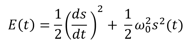
The Foundation: Volatility
The Catapult predicts significant changes with the 21-period Relative Volatility Index.
The Average True Range, Mean Absolute Deviation, and Standard Deviation all assess volatility. Standard Deviation will construct the Relative Volatility Index.
Standard Deviation is the most basic volatility. It underpins descriptive statistics and technical indicators like Bollinger Bands. Before calculating Standard Deviation, let's define Variance.
Variance is the squared deviations from the mean (a dispersion measure). We take the square deviations to compel the distance from the mean to be non-negative, then we take the square root to make the measure have the same units as the mean, comparing apples to apples (mean to standard deviation standard deviation). Variance formula:
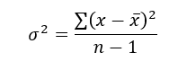
As stated, standard deviation is:
# The function to add a number of columns inside an array
def adder(Data, times):

    for i in range(1, times + 1):

        new_col = np.zeros((len(Data), 1), dtype = float)
        Data = np.append(Data, new_col, axis = 1)

    return Data

# The function to delete a number of columns starting from an index
def deleter(Data, index, times):

    for i in range(1, times + 1):

        Data = np.delete(Data, index, axis = 1)

    return Data

# The function to delete a number of rows from the beginning
def jump(Data, jump):

    Data = Data[jump:, ]

    return Data

# Example of adding 3 empty columns to an array
my_ohlc_array = adder(my_ohlc_array, 3)

# Example of deleting the 2 columns after the column indexed at 3
my_ohlc_array = deleter(my_ohlc_array, 3, 2)

# Example of deleting the first 20 rows
my_ohlc_array = jump(my_ohlc_array, 20)

# Remember, OHLC is an abbreviation of Open, High, Low, and Close and it refers to the standard historical data file

def volatility(Data, lookback, what, where):

  for i in range(len(Data)):

     try:

        Data[i, where] = (Data[i - lookback + 1:i + 1, what].std())
     except IndexError:
        pass

  return Data
The RSI is the most popular momentum indicator, and for good reason—it excels in range markets. Its 0–100 range simplifies interpretation. Fame boosts its potential.
The more traders and portfolio managers look at the RSI, the more people will react to its signals, pushing market prices. Technical Analysis is self-fulfilling, therefore this theory is obvious yet unproven.
RSI is determined simply. Start with one-period pricing discrepancies. We must remove each closing price from the previous one. We then divide the smoothed average of positive differences by the smoothed average of negative differences. The RSI algorithm converts the Relative Strength from the last calculation into a value between 0 and 100.
def ma(Data, lookback, close, where):
Data = adder(Data, 1)
for i in range(len(Data)):
try:
Data[i, where] = (Data[i - lookback + 1:i + 1, close].mean())
except IndexError:
pass
# Cleaning
Data = jump(Data, lookback)
return Data
def ema(Data, alpha, lookback, what, where):
alpha = alpha / (lookback + 1.0)
beta = 1 - alpha
# First value is a simple SMA
Data = ma(Data, lookback, what, where)
# Calculating first EMA
Data[lookback + 1, where] = (Data[lookback + 1, what] * alpha) + (Data[lookback, where] * beta)
# Calculating the rest of EMA
for i in range(lookback + 2, len(Data)):
try:
Data[i, where] = (Data[i, what] * alpha) + (Data[i - 1, where] * beta)
except IndexError:
pass
return Datadef rsi(Data, lookback, close, where, width = 1, genre = 'Smoothed'):
# Adding a few columns
Data = adder(Data, 7)
# Calculating Differences
for i in range(len(Data)):
Data[i, where] = Data[i, close] - Data[i - width, close]
# Calculating the Up and Down absolute values
for i in range(len(Data)):
if Data[i, where] > 0:
Data[i, where + 1] = Data[i, where]
elif Data[i, where] < 0:
Data[i, where + 2] = abs(Data[i, where])
# Calculating the Smoothed Moving Average on Up and Down
absolute values
lookback = (lookback * 2) - 1 # From exponential to smoothed
Data = ema(Data, 2, lookback, where + 1, where + 3)
Data = ema(Data, 2, lookback, where + 2, where + 4)
# Calculating the Relative Strength
Data[:, where + 5] = Data[:, where + 3] / Data[:, where + 4]
# Calculate the Relative Strength Index
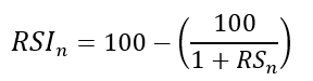
Data[:, where + 6] = (100 - (100 / (1 + Data[:, where + 5])))
# Cleaning
Data = deleter(Data, where, 6)
Data = jump(Data, lookback)
return Data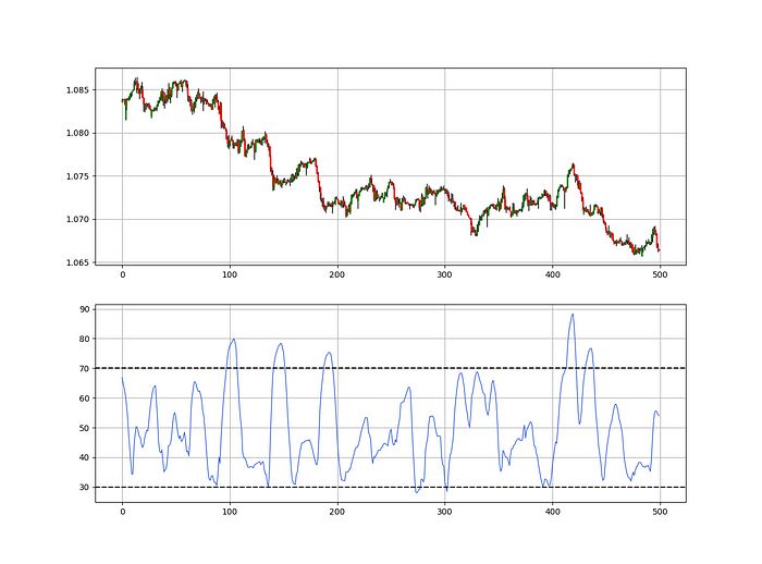
def relative_volatility_index(Data, lookback, close, where):

    # Calculating Volatility
    Data = volatility(Data, lookback, close, where)

    # Calculating the RSI on Volatility
    Data = rsi(Data, lookback, where, where + 1)

    # Cleaning
    Data = deleter(Data, where, 1)

    return Data
The Arm Section: Speed
The Catapult predicts momentum direction using the 14-period Relative Strength Index.
As a reminder, the RSI ranges from 0 to 100. Two levels give contrarian signals:
A positive response is anticipated when the market is deemed to have gone too far down at the oversold level 30, which is 30.
When the market is deemed to have gone up too much, at overbought level 70, a bearish reaction is to be expected.
Comparing the RSI to 50 is another intriguing use. RSI above 50 indicates bullish momentum, while below 50 indicates negative momentum.
The direction-finding filter in the frame
The Catapult's directional filter uses the 200-period simple moving average to keep us trending. This keeps us sane and increases our odds.
Moving averages confirm and ride trends. Its simplicity and track record of delivering value to analysis make them the most popular technical indicator. They help us locate support and resistance, stops and targets, and the trend. Its versatility makes them essential trading tools.
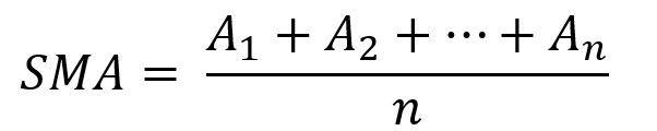
This is the plain mean, employed in statistics and everywhere else in life. Simply divide the number of observations by their total values. Mathematically, it's:
We defined the moving average function above. Create the Catapult indication now.
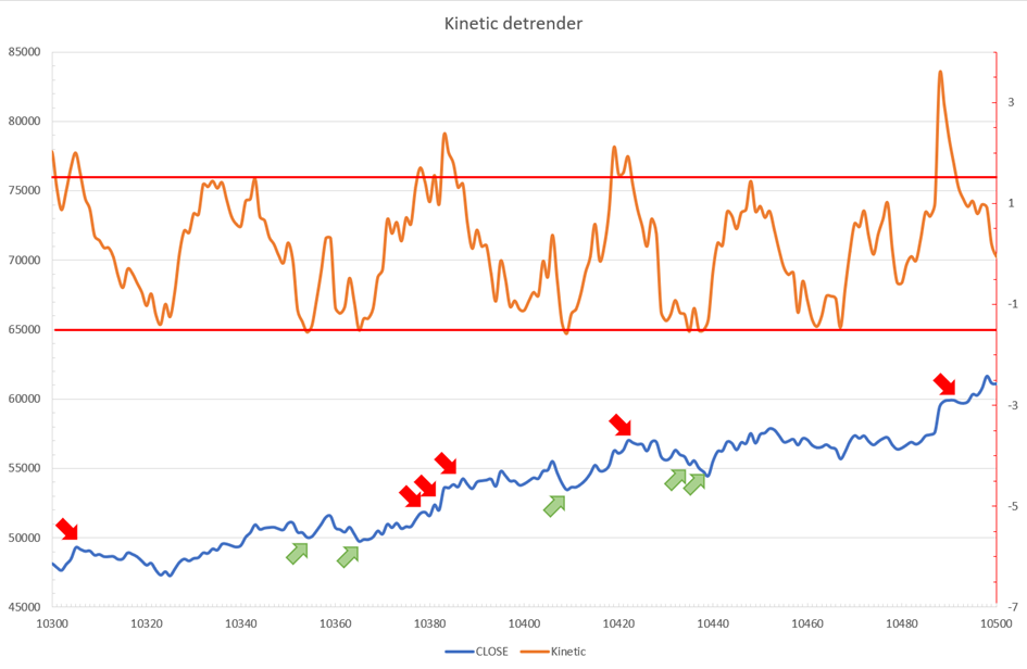
Indicator of the Catapult
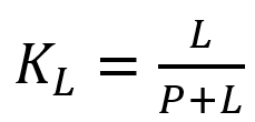
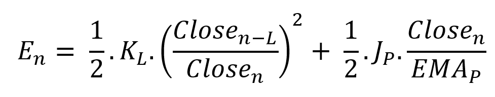
The indicator is a healthy mix of the three indicators:
The first trigger will be provided by the 21-period Relative Volatility Index, which indicates that there will now be above average volatility and, as a result, it is possible for a directional shift.
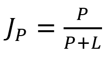
If the reading is above 50, the move is likely bullish, and if it is below 50, the move is likely bearish, according to the 14-period Relative Strength Index, which indicates the likelihood of the direction of the move.
The likelihood of the move's direction will be strengthened by the 200-period simple moving average. When the market is above the 200-period moving average, we can infer that bullish pressure is there and that the upward trend will likely continue. Similar to this, if the market falls below the 200-period moving average, we recognize that there is negative pressure and that the downside is quite likely to continue.
lookback_rvi = 21
lookback_rsi = 14
lookback_ma = 200
my_data = ma(my_data, lookback_ma, 3, 4)
my_data = rsi(my_data, lookback_rsi, 3, 5)
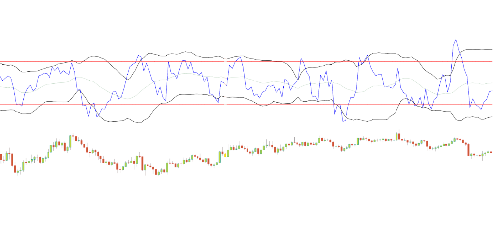
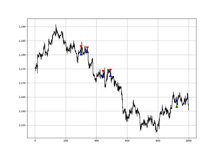
my_data = relative_volatility_index(my_data, lookback_rvi, 3, 6)Two-handled overlay indicator Catapult. The first exhibits blue and green arrows for a buy signal, and the second shows blue and red for a sell signal.
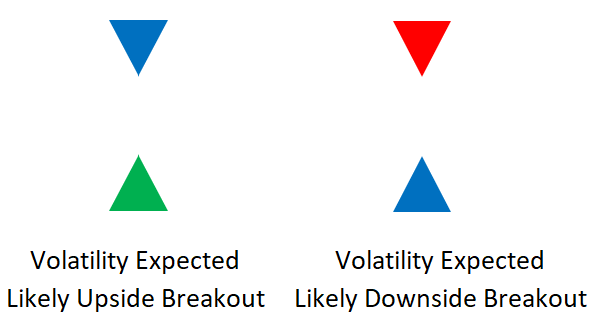
The chart below shows recent EURUSD hourly values.
def signal(Data, rvi_col, signal):

    Data = adder(Data, 10)

    for i in range(len(Data)):

        if Data[i,     rvi_col] < 30 and \
           Data[i - 1, rvi_col] > 30 and \
           Data[i - 2, rvi_col] > 30 and \
           Data[i - 3, rvi_col] > 30 and \
           Data[i - 4, rvi_col] > 30 and \
           Data[i - 5, rvi_col] > 30:

               Data[i, signal] = 1

    return Data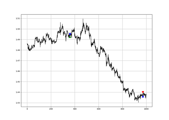
Signals are straightforward. The indicator can be utilized with other methods.
my_data = signal(my_data, 6, 7)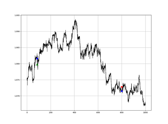
Lumiwealth shows how to develop all kinds of algorithms. I recommend their hands-on courses in algorithmic trading, blockchain, and machine learning.
Summary
To conclude, my goal is to contribute to objective technical analysis, which promotes more transparent methods and strategies that must be back-tested before implementation. Technical analysis will lose its reputation as subjective and unscientific.
After you find a trading method or approach, follow these steps:
Put emotions aside and adopt an analytical perspective.
Test it in the past in conditions and simulations taken from real life.
Try improving it and performing a forward test if you notice any possibility.
Transaction charges and any slippage simulation should always be included in your tests.
Risk management and position sizing should always be included in your tests.
After checking the aforementioned, monitor the plan because market dynamics may change and render it unprofitable.

Ray Dalio
3 years ago
The latest “bubble indicator” readings.
As you know, I like to turn my intuition into decision rules (principles) that can be back-tested and automated to create a portfolio of alpha bets. I use one for bubbles. Having seen many bubbles in my 50+ years of investing, I described what makes a bubble and how to identify them in markets—not just stocks.
A bubble market has a high degree of the following:
- High prices compared to traditional values (e.g., by taking the present value of their cash flows for the duration of the asset and comparing it with their interest rates).
- Conditons incompatible with long-term growth (e.g., extrapolating past revenue and earnings growth rates late in the cycle).
- Many new and inexperienced buyers were drawn in by the perceived hot market.
- Broad bullish sentiment.
- Debt financing a large portion of purchases.
- Lots of forward and speculative purchases to profit from price rises (e.g., inventories that are more than needed, contracted forward purchases, etc.).
I use these criteria to assess all markets for bubbles. I have periodically shown you these for stocks and the stock market.
What Was Shown in January Versus Now
I will first describe the picture in words, then show it in charts, and compare it to the last update in January.
As of January, the bubble indicator showed that a) the US equity market was in a moderate bubble, but not an extreme one (ie., 70 percent of way toward the highest bubble, which occurred in the late 1990s and late 1920s), and b) the emerging tech companies (ie. As well, the unprecedented flood of liquidity post-COVID financed other bubbly behavior (e.g. SPACs, IPO boom, big pickup in options activity), making things bubbly. I showed which stocks were in bubbles and created an index of those stocks, which I call “bubble stocks.”
Those bubble stocks have popped. They fell by a third last year, while the S&P 500 remained flat. In light of these and other market developments, it is not necessarily true that now is a good time to buy emerging tech stocks.
The fact that they aren't at a bubble extreme doesn't mean they are safe or that it's a good time to get long. Our metrics still show that US stocks are overvalued. Once popped, bubbles tend to overcorrect to the downside rather than settle at “normal” prices.
The following charts paint the picture. The first shows the US equity market bubble gauge/indicator going back to 1900, currently at the 40% percentile. The charts also zoom in on the gauge in recent years, as well as the late 1920s and late 1990s bubbles (during both of these cases the gauge reached 100 percent ).
The chart below depicts the average bubble gauge for the most bubbly companies in 2020. Those readings are down significantly.
The charts below compare the performance of a basket of emerging tech bubble stocks to the S&P 500. Prices have fallen noticeably, giving up most of their post-COVID gains.
The following charts show the price action of the bubble slice today and in the 1920s and 1990s. These charts show the same market dynamics and two key indicators. These are just two examples of how a lot of debt financing stock ownership coupled with a tightening typically leads to a bubble popping.
Everything driving the bubbles in this market segment is classic—the same drivers that drove the 1920s bubble and the 1990s bubble. For instance, in the last couple months, it was how tightening can act to prick the bubble. Review this case study of the 1920s stock bubble (starting on page 49) from my book Principles for Navigating Big Debt Crises to grasp these dynamics.
The following charts show the components of the US stock market bubble gauge. Since this is a proprietary indicator, I will only show you some of the sub-aggregate readings and some indicators.
Each of these six influences is measured using a number of stats. This is how I approach the stock market. These gauges are combined into aggregate indices by security and then for the market as a whole. The table below shows the current readings of these US equity market indicators. It compares current conditions for US equities to historical conditions. These readings suggest that we’re out of a bubble.
1. How High Are Prices Relatively?
This price gauge for US equities is currently around the 50th percentile.
2. Is price reduction unsustainable?
This measure calculates the earnings growth rate required to outperform bonds. This is calculated by adding up the readings of individual securities. This indicator is currently near the 60th percentile for the overall market, higher than some of our other readings. Profit growth discounted in stocks remains high.
Even more so in the US software sector. Analysts' earnings growth expectations for this sector have slowed, but remain high historically. P/Es have reversed COVID gains but remain high historical.
3. How many new buyers (i.e., non-existing buyers) entered the market?
Expansion of new entrants is often indicative of a bubble. According to historical accounts, this was true in the 1990s equity bubble and the 1929 bubble (though our data for this and other gauges doesn't go back that far). A flood of new retail investors into popular stocks, which by other measures appeared to be in a bubble, pushed this gauge above the 90% mark in 2020. The pace of retail activity in the markets has recently slowed to pre-COVID levels.
4. How Broadly Bullish Is Sentiment?
The more people who have invested, the less resources they have to keep investing, and the more likely they are to sell. Market sentiment is now significantly negative.
5. Are Purchases Being Financed by High Leverage?
Leveraged purchases weaken the buying foundation and expose it to forced selling in a downturn. The leverage gauge, which considers option positions as a form of leverage, is now around the 50% mark.
6. To What Extent Have Buyers Made Exceptionally Extended Forward Purchases?
Looking at future purchases can help assess whether expectations have become overly optimistic. This indicator is particularly useful in commodity and real estate markets, where forward purchases are most obvious. In the equity markets, I look at indicators like capital expenditure, or how much businesses (and governments) invest in infrastructure, factories, etc. It reflects whether businesses are projecting future demand growth. Like other gauges, this one is at the 40th percentile.
What one does with it is a tactical choice. While the reversal has been significant, future earnings discounting remains high historically. In either case, bubbles tend to overcorrect (sell off more than the fundamentals suggest) rather than simply deflate. But I wanted to share these updated readings with you in light of recent market activity.
Sofien Kaabar, CFA
3 years ago
How to Make a Trading Heatmap
Python Heatmap Technical Indicator

Heatmaps provide an instant overview. They can be used with correlations or to predict reactions or confirm the trend in trading. This article covers RSI heatmap creation.
The Market System
Market regime:
Bullish trend: The market tends to make higher highs, which indicates that the overall trend is upward.
Sideways: The market tends to fluctuate while staying within predetermined zones.
Bearish trend: The market has the propensity to make lower lows, indicating that the overall trend is downward.
Most tools detect the trend, but we cannot predict the next state. The best way to solve this problem is to assume the current state will continue and trade any reactions, preferably in the trend.
If the EURUSD is above its moving average and making higher highs, a trend-following strategy would be to wait for dips before buying and assuming the bullish trend will continue.
Indicator of Relative Strength
J. Welles Wilder Jr. introduced the RSI, a popular and versatile technical indicator. Used as a contrarian indicator to exploit extreme reactions. Calculating the default RSI usually involves these steps:
Determine the difference between the closing prices from the prior ones.
Distinguish between the positive and negative net changes.
Create a smoothed moving average for both the absolute values of the positive net changes and the negative net changes.
Take the difference between the smoothed positive and negative changes. The Relative Strength RS will be the name we use to describe this calculation.
To obtain the RSI, use the normalization formula shown below for each time step.
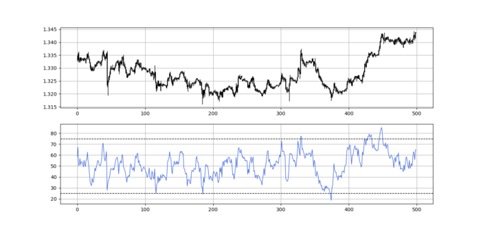
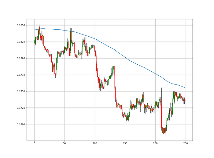
The 13-period RSI and black GBPUSD hourly values are shown above. RSI bounces near 25 and pauses around 75. Python requires a four-column OHLC array for RSI coding.
import numpy as np
def add_column(data, times):

    for i in range(1, times + 1):

        new = np.zeros((len(data), 1), dtype = float)

        data = np.append(data, new, axis = 1)
    return data
def delete_column(data, index, times):

    for i in range(1, times + 1):

        data = np.delete(data, index, axis = 1)
    return data
def delete_row(data, number):

    data = data[number:, ]

    return data
def ma(data, lookback, close, position):

    data = add_column(data, 1)

    for i in range(len(data)):

            try:

                data[i, position] = (data[i - lookback + 1:i + 1, close].mean())

            except IndexError:

                pass

    data = delete_row(data, lookback)

    return data
def smoothed_ma(data, alpha, lookback, close, position):

    lookback = (2 * lookback) - 1

    alpha = alpha / (lookback + 1.0)

    beta  = 1 - alpha

    data = ma(data, lookback, close, position)
    data[lookback + 1, position] = (data[lookback + 1, close] * alpha) + (data[lookback, position] * beta)
    for i in range(lookback + 2, len(data)):

            try:

                data[i, position] = (data[i, close] * alpha) + (data[i - 1, position] * beta)

            except IndexError:

                pass

    return data
def rsi(data, lookback, close, position):

    data = add_column(data, 5)

    for i in range(len(data)):

        data[i, position] = data[i, close] - data[i - 1, close]

    for i in range(len(data)):

        if data[i, position] > 0:

            data[i, position + 1] = data[i, position]

        elif data[i, position] < 0:

            data[i, position + 2] = abs(data[i, position])

    data = smoothed_ma(data, 2, lookback, position + 1, position + 3)
    data = smoothed_ma(data, 2, lookback, position + 2, position + 4)
    data[:, position + 5] = data[:, position + 3] / data[:, position + 4]

    data[:, position + 6] = (100 - (100 / (1 + data[:, position + 5])))
    data = delete_column(data, position, 6)
    data = delete_row(data, lookback)
    return data
Make sure to focus on the concepts and not the code. You can find the codes of most of my strategies in my books. The most important thing is to comprehend the techniques and strategies.
My weekly market sentiment report uses complex and simple models to understand the current positioning and predict the future direction of several major markets. Check out the report here:
Using the Heatmap to Find the Trend
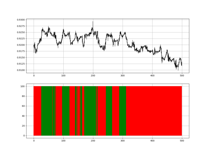
RSI trend detection is easy but useless. Bullish and bearish regimes are in effect when the RSI is above or below 50, respectively. Tracing a vertical colored line creates the conditions below. How:
When the RSI is higher than 50, a green vertical line is drawn.
When the RSI is lower than 50, a red vertical line is drawn.
Zooming out yields a basic heatmap, as shown below.
Plot code:
def indicator_plot(data, second_panel, window = 250):
    fig, ax = plt.subplots(2, figsize = (10, 5))
    sample = data[-window:, ]
    for i in range(len(sample)):
        ax[0].vlines(x = i, ymin = sample[i, 2], ymax = sample[i, 1], color = 'black', linewidth = 1)
        if sample[i, 3] > sample[i, 0]:
            ax[0].vlines(x = i, ymin = sample[i, 0], ymax = sample[i, 3], color = 'black', linewidth = 1.5)
        if sample[i, 3] < sample[i, 0]:
            ax[0].vlines(x = i, ymin = sample[i, 3], ymax = sample[i, 0], color = 'black', linewidth = 1.5)
        if sample[i, 3] == sample[i, 0]:
            ax[0].vlines(x = i, ymin = sample[i, 3], ymax = sample[i, 0], color = 'black', linewidth = 1.5)
    ax[0].grid()
    for i in range(len(sample)):
        if sample[i, second_panel] > 50:
            ax[1].vlines(x = i, ymin = 0, ymax = 100, color = 'green', linewidth = 1.5)
        if sample[i, second_panel] < 50:
            ax[1].vlines(x = i, ymin = 0, ymax = 100, color = 'red', linewidth = 1.5)
    ax[1].grid()
indicator_plot(my_data, 4, window = 500)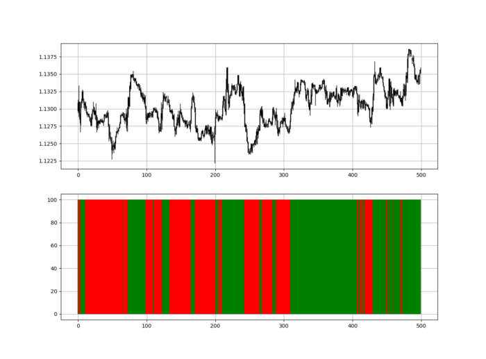
Call RSI on your OHLC array's fifth column. 4. Adjusting lookback parameters reduces lag and false signals. Other indicators and conditions are possible.
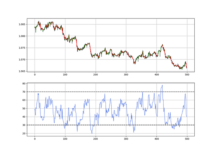
Another suggestion is to develop an RSI Heatmap for Extreme Conditions.
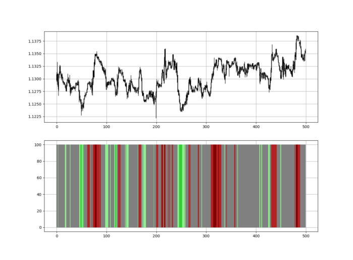
Contrarian indicator RSI. The following rules apply:
Whenever the RSI is approaching the upper values, the color approaches red.
The color tends toward green whenever the RSI is getting close to the lower values.
Zooming out yields a basic heatmap, as shown below.
Plot code:
import matplotlib.pyplot as plt
def indicator_plot(data, second_panel, window = 250):
    fig, ax = plt.subplots(2, figsize = (10, 5))
    sample = data[-window:, ]
    for i in range(len(sample)):
        ax[0].vlines(x = i, ymin = sample[i, 2], ymax = sample[i, 1], color = 'black', linewidth = 1)
        if sample[i, 3] > sample[i, 0]:
            ax[0].vlines(x = i, ymin = sample[i, 0], ymax = sample[i, 3], color = 'black', linewidth = 1.5)
        if sample[i, 3] < sample[i, 0]:
            ax[0].vlines(x = i, ymin = sample[i, 3], ymax = sample[i, 0], color = 'black', linewidth = 1.5)
        if sample[i, 3] == sample[i, 0]:
            ax[0].vlines(x = i, ymin = sample[i, 3], ymax = sample[i, 0], color = 'black', linewidth = 1.5)
    ax[0].grid()
    for i in range(len(sample)):
        if sample[i, second_panel] > 90:
            ax[1].vlines(x = i, ymin = 0, ymax = 100, color = 'red', linewidth = 1.5)
        if sample[i, second_panel] > 80 and sample[i, second_panel] < 90:
            ax[1].vlines(x = i, ymin = 0, ymax = 100, color = 'darkred', linewidth = 1.5)
        if sample[i, second_panel] > 70 and sample[i, second_panel] < 80:
            ax[1].vlines(x = i, ymin = 0, ymax = 100, color = 'maroon', linewidth = 1.5)
        if sample[i, second_panel] > 60 and sample[i, second_panel] < 70:
            ax[1].vlines(x = i, ymin = 0, ymax = 100, color = 'firebrick', linewidth = 1.5)
        if sample[i, second_panel] > 50 and sample[i, second_panel] < 60:
            ax[1].vlines(x = i, ymin = 0, ymax = 100, color = 'grey', linewidth = 1.5)
        if sample[i, second_panel] > 40 and sample[i, second_panel] < 50:
            ax[1].vlines(x = i, ymin = 0, ymax = 100, color = 'grey', linewidth = 1.5)
        if sample[i, second_panel] > 30 and sample[i, second_panel] < 40:
            ax[1].vlines(x = i, ymin = 0, ymax = 100, color = 'lightgreen', linewidth = 1.5)
        if sample[i, second_panel] > 20 and sample[i, second_panel] < 30:
            ax[1].vlines(x = i, ymin = 0, ymax = 100, color = 'limegreen', linewidth = 1.5)
        if sample[i, second_panel] > 10 and sample[i, second_panel] < 20:
            ax[1].vlines(x = i, ymin = 0, ymax = 100, color = 'seagreen', linewidth = 1.5)
        if sample[i, second_panel] > 0 and sample[i, second_panel] < 10:
            ax[1].vlines(x = i, ymin = 0, ymax = 100, color = 'green', linewidth = 1.5)
    ax[1].grid()
indicator_plot(my_data, 4, window = 500)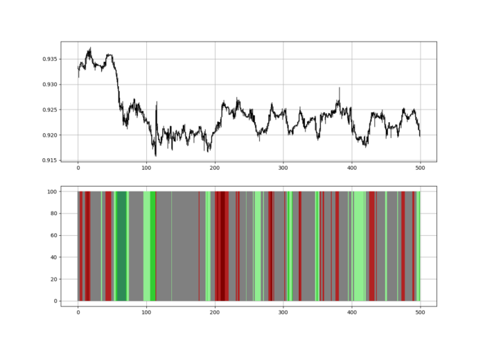
Dark green and red areas indicate imminent bullish and bearish reactions, respectively. RSI around 50 is grey.
Summary
To conclude, my goal is to contribute to objective technical analysis, which promotes more transparent methods and strategies that must be back-tested before implementation.
Technical analysis will lose its reputation as subjective and unscientific.
When you find a trading strategy or technique, follow these steps:
Put emotions aside and adopt a critical mindset.
Test it in the past under conditions and simulations taken from real life.
Try optimizing it and performing a forward test if you find any potential.
Transaction costs and any slippage simulation should always be included in your tests.
Risk management and position sizing should always be considered in your tests.
After checking the above, monitor the strategy because market dynamics may change and make it unprofitable.
You might also like

CyberPunkMetalHead
3 years ago
195 countries want Terra Luna founder Do Kwon
Interpol has issued a red alert on Terraform Labs' CEO, South Korean prosecutors said.

After the May crash of Terra Luna revealed tax evasion issues, South Korean officials filed an arrest warrant for Do Kwon, but he is missing.
Do Kwon is now a fugitive in 195 countries after Seoul prosecutors placed him to Interpol's red list. Do Kwon hasn't commented since then. The red list allows any country's local authorities to apprehend Do Kwon.
Do Dwon and Terraform Labs were believed to have moved to Singapore days before the $40 billion wipeout, but Singapore authorities said he fled the country on September 17. Do Kwon tweeted that he wasn't on the run and cited privacy concerns.
Do Kwon was not on the red list at the time and said he wasn't "running," only to reply to his own tweet saying he hasn't jogged in a while and needed to trim calories.
Whether or not it makes sense to read too much into this, the reality is that Do Kwon is now on Interpol red list, despite the firmly asserts on twitter that he does absolutely nothing to hide.
UPDATE:
South Korean authorities are investigating alleged withdrawals of over $60 million U.S. and seeking to freeze these assets. Korean authorities believe a new wallet exchanged over 3000 BTC through OKX and Kucoin.
Do Kwon and the Luna Foundation Guard (of whom Do Kwon is a key member of) have declined all charges and dubbed this disinformation.
Singapore's Luna Foundation Guard (LFG) manages the Terra Ecosystem.
The Legal Situation
Multiple governments are searching for Do Kwon and five other Terraform Labs employees for financial markets legislation crimes.
South Korean authorities arrested a man suspected of tax fraud and Ponzi scheme.
The U.S. SEC is also examining Terraform Labs on how UST was advertised as a stablecoin. No legal precedent exists, so it's unclear what's illegal.
The future of Terraform Labs, Terra, and Terra 2 is unknown, and despite what Twitter shills say about LUNC, the company remains in limbo awaiting a decision that will determine its fate. This project isn't a wise investment.

Scott Stockdale
3 years ago
A Day in the Life of Lex Fridman Can Help You Hit 6-Month Goals

The Lex Fridman podcast host has interviewed Elon Musk.
Lex is a minimalist YouTuber. His videos are sloppy. Suits are his trademark.
In a video, he shares a typical day. I've smashed my 6-month goals using its ideas.
Here's his schedule.
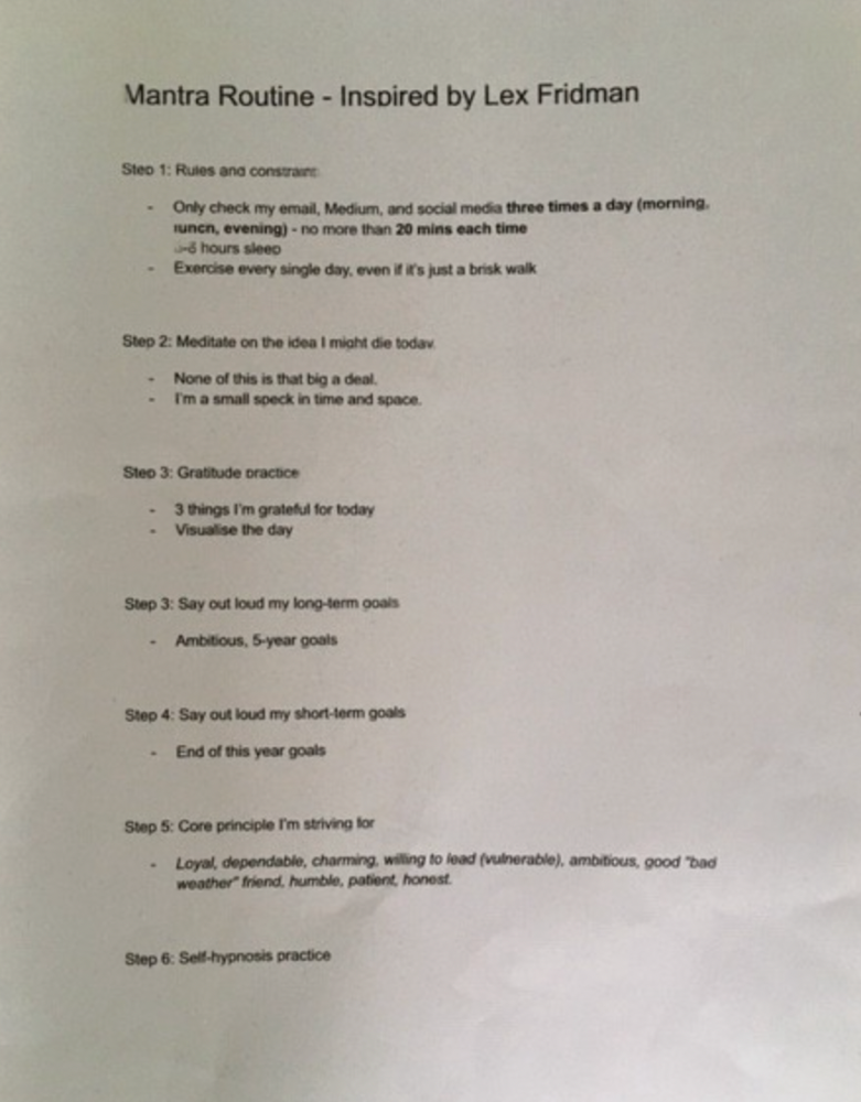
Morning Mantra
Not woo-woo. Lex's mantra reflects his practicality.
Four parts.
Rulebook
"I remember the game's rules," he says.
Among them:
Sleeping 6–8 hours nightly
1–3 times a day, he checks social media.
Every day, despite pain, he exercises. "I exercise uninjured body parts."
Visualize
He imagines his day. "Like Sims..."
He says three things he's grateful for and contemplates death.
"Today may be my last"
Objectives
Then he visualizes his goals. He starts big. Five-year goals.
Short-term goals follow. Lex says they're year-end goals.
Near but out of reach.
Principles
He lists his principles. Assertions. His goals.
He acknowledges his cliche beliefs. Compassion, empathy, and strength are key.
Here's my mantra routine:
Four-Hour Deep Work
Lex begins a four-hour deep work session after his mantra routine. Today's toughest.
AI is Lex's specialty. His video doesn't explain what he does.
Clearly, he works hard.
Before starting, he has water, coffee, and a bathroom break.
"During deep work sessions, I minimize breaks."
He's distraction-free. Phoneless. Silence. Nothing. Any loose ideas are typed into a Google doc for later. He wants to work.
"Just get the job done. Don’t think about it too much and feel good once it’s complete." — Lex Fridman
30-Minute Social Media & Music
After his first deep work session, Lex rewards himself.
10 minutes on social media, 20 on music. Upload content and respond to comments in 10 minutes. 20 minutes for guitar or piano.
"In the real world, I’m currently single, but in the music world, I’m in an open relationship with this beautiful guitar. Open relationship because sometimes I cheat on her with the acoustic." — Lex Fridman
Two-hour exercise
Then exercise for two hours.
Daily runs six miles. Then he chooses how far to go. Run time is an hour.
He does bodyweight exercises. Every minute for 15 minutes, do five pull-ups and ten push-ups. It's David Goggins-inspired. He aims for an hour a day.
He's hungry. Before running, he takes a salt pill for electrolytes.
He'll then take a one-minute cold shower while listening to cheesy songs. Afterward, he might eat.
Four-Hour Deep Work
Lex's second work session.
He works 8 hours a day.
Again, zero distractions.
Eating
The video's meal doesn't look appetizing, but it's healthy.
It's ground beef with vegetables. Cauliflower is his "ground-floor" veggie. "Carrots are my go-to party food."
Lex's keto diet includes 1800–2000 calories.
He drinks a "nutrient-packed" Atheltic Greens shake and takes tablets. It's:
One daily tablet of sodium.
Magnesium glycinate tablets stopped his keto headaches.
Potassium — "For electrolytes"
Fish oil: healthy joints
“So much of nutrition science is barely a science… I like to listen to my own body and do a one-person, one-subject scientific experiment to feel good.” — Lex Fridman
Four-hour shallow session
This work isn't as mentally taxing.
Lex planned to:
Finish last session's deep work (about an hour)
Adobe Premiere podcasting (about two hours).
Email-check (about an hour). Three times a day max. First, check for emergencies.
If he's sick, he may watch Netflix or YouTube documentaries or visit friends.
“The possibilities of chaos are wide open, so I can do whatever the hell I want.” — Lex Fridman
Two-hour evening reading
Nonstop work.
Lex ends the day reading academic papers for an hour. "Today I'm skimming two machine learning and neuroscience papers"
This helps him "think beyond the paper."
He reads for an hour.
“When I have a lot of energy, I just chill on the bed and read… When I’m feeling tired, I jump to the desk…” — Lex Fridman
Takeaways
Lex's day-in-the-life video is inspiring.
He has positive energy and works hard every day.
Schedule:
Mantra Routine includes rules, visualizing, goals, and principles.
Deep Work Session #1: Four hours of focus.
10 minutes social media, 20 minutes guitar or piano. "Music brings me joy"
Six-mile run, then bodyweight workout. Two hours total.
Deep Work #2: Four hours with no distractions. Google Docs stores random thoughts.
Lex supplements his keto diet.
This four-hour session is "open to chaos."
Evening reading: academic papers followed by fiction.
"I value some things in life. Work is one. The other is loving others. With those two things, life is great." — Lex Fridman

Hasan AboulHasan
3 years ago
High attachment products can help you earn money automatically.

Affiliate marketing is a popular online moneymaker. You promote others' products and get commissions. Affiliate marketing requires constant product promotion.
Affiliate marketing can be profitable even without much promotion. Yes, this is Autopilot Money.
How to Pick an Affiliate Program to Generate Income Autonomously
Autopilot moneymaking requires a recurring affiliate marketing program.
Finding the best product and testing it takes a lot of time and effort.
Here are three ways to choose the best service or product to promote:
Find a good attachment-rate product or service.
When choosing a product, ask if you can easily switch to another service. Attachment rate is how much people like a product.
Higher attachment rates mean better Autopilot products.
Consider promoting GetResponse. It's a 33% recurring commission email marketing tool. This means you get 33% of the customer's plan as long as he pays.
GetResponse has a high attachment rate because it's hard to leave and start over with another tool.
2. Pick a good or service with a lot of affiliate assets.
Check if a program has affiliate assets or creatives before joining.
Images and banners to promote the product in your business.
They save time; I look for promotional creatives. Creatives or affiliate assets are website banners or images. This reduces design time.
3. Select a service or item that consumers already adore.
New products are hard to sell. Choosing a trusted company's popular product or service is helpful.
As a beginner, let people buy a product they already love.
Online entrepreneurs and digital marketers love Systeme.io. It offers tools for creating pages, email marketing, funnels, and more. This product guarantees a high ROI.
Make the product known!
Affiliate marketers struggle to get traffic. Using affiliate marketing to make money is easier than you think if you have a solid marketing strategy.
Your plan should include:
1- Publish affiliate-related blog posts and SEO-optimize them
2- Sending new visitors product-related emails
3- Create a product resource page.
4-Review products
5-Make YouTube videos with links in the description.
6- Answering FAQs about your products and services on your blog and Quora.
7- Create an eCourse on how to use this product.
8- Adding Affiliate Banners to Your Website.
With these tips, you can promote your products and make money on autopilot.