


More on Economics & Investing
Wayne Duggan
3 years ago
What An Inverted Yield Curve Means For Investors
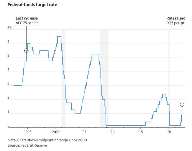
The yield spread between 10-year and 2-year US Treasury bonds has fallen below 0.2 percent, its lowest level since March 2020. A flattening or negative yield curve can be a bad sign for the economy.
What Is An Inverted Yield Curve?
In the yield curve, bonds of equal credit quality but different maturities are plotted. The most commonly used yield curve for US investors is a plot of 2-year and 10-year Treasury yields, which have yet to invert.
A typical yield curve has higher interest rates for future maturities. In a flat yield curve, short-term and long-term yields are similar. Inverted yield curves occur when short-term yields exceed long-term yields. Inversions of yield curves have historically occurred during recessions.
Inverted yield curves have preceded each of the past eight US recessions. The good news is they're far leading indicators, meaning a recession is likely not imminent.
Every US recession since 1955 has occurred between six and 24 months after an inversion of the two-year and 10-year Treasury yield curves, according to the San Francisco Fed. So, six months before COVID-19, the yield curve inverted in August 2019.
Looking Ahead
The spread between two-year and 10-year Treasury yields was 0.18 percent on Tuesday, the smallest since before the last US recession. If the graph above continues, a two-year/10-year yield curve inversion could occur within the next few months.
According to Bank of America analyst Stephen Suttmeier, the S&P 500 typically peaks six to seven months after the 2s-10s yield curve inverts, and the US economy enters recession six to seven months later.
Investors appear unconcerned about the flattening yield curve. This is in contrast to the iShares 20+ Year Treasury Bond ETF TLT +2.19% which was down 1% on Tuesday.
Inversion of the yield curve and rising interest rates have historically harmed stocks. Recessions in the US have historically coincided with or followed the end of a Federal Reserve rate hike cycle, not the start.
Ray Dalio
3 years ago
The latest “bubble indicator” readings.
As you know, I like to turn my intuition into decision rules (principles) that can be back-tested and automated to create a portfolio of alpha bets. I use one for bubbles. Having seen many bubbles in my 50+ years of investing, I described what makes a bubble and how to identify them in markets—not just stocks.
A bubble market has a high degree of the following:
- High prices compared to traditional values (e.g., by taking the present value of their cash flows for the duration of the asset and comparing it with their interest rates).
- Conditons incompatible with long-term growth (e.g., extrapolating past revenue and earnings growth rates late in the cycle).
- Many new and inexperienced buyers were drawn in by the perceived hot market.
- Broad bullish sentiment.
- Debt financing a large portion of purchases.
- Lots of forward and speculative purchases to profit from price rises (e.g., inventories that are more than needed, contracted forward purchases, etc.).
I use these criteria to assess all markets for bubbles. I have periodically shown you these for stocks and the stock market.
What Was Shown in January Versus Now
I will first describe the picture in words, then show it in charts, and compare it to the last update in January.
As of January, the bubble indicator showed that a) the US equity market was in a moderate bubble, but not an extreme one (ie., 70 percent of way toward the highest bubble, which occurred in the late 1990s and late 1920s), and b) the emerging tech companies (ie. As well, the unprecedented flood of liquidity post-COVID financed other bubbly behavior (e.g. SPACs, IPO boom, big pickup in options activity), making things bubbly. I showed which stocks were in bubbles and created an index of those stocks, which I call “bubble stocks.”
Those bubble stocks have popped. They fell by a third last year, while the S&P 500 remained flat. In light of these and other market developments, it is not necessarily true that now is a good time to buy emerging tech stocks.
The fact that they aren't at a bubble extreme doesn't mean they are safe or that it's a good time to get long. Our metrics still show that US stocks are overvalued. Once popped, bubbles tend to overcorrect to the downside rather than settle at “normal” prices.
The following charts paint the picture. The first shows the US equity market bubble gauge/indicator going back to 1900, currently at the 40% percentile. The charts also zoom in on the gauge in recent years, as well as the late 1920s and late 1990s bubbles (during both of these cases the gauge reached 100 percent ).
The chart below depicts the average bubble gauge for the most bubbly companies in 2020. Those readings are down significantly.
The charts below compare the performance of a basket of emerging tech bubble stocks to the S&P 500. Prices have fallen noticeably, giving up most of their post-COVID gains.
The following charts show the price action of the bubble slice today and in the 1920s and 1990s. These charts show the same market dynamics and two key indicators. These are just two examples of how a lot of debt financing stock ownership coupled with a tightening typically leads to a bubble popping.
Everything driving the bubbles in this market segment is classic—the same drivers that drove the 1920s bubble and the 1990s bubble. For instance, in the last couple months, it was how tightening can act to prick the bubble. Review this case study of the 1920s stock bubble (starting on page 49) from my book Principles for Navigating Big Debt Crises to grasp these dynamics.
The following charts show the components of the US stock market bubble gauge. Since this is a proprietary indicator, I will only show you some of the sub-aggregate readings and some indicators.
Each of these six influences is measured using a number of stats. This is how I approach the stock market. These gauges are combined into aggregate indices by security and then for the market as a whole. The table below shows the current readings of these US equity market indicators. It compares current conditions for US equities to historical conditions. These readings suggest that we’re out of a bubble.
1. How High Are Prices Relatively?
This price gauge for US equities is currently around the 50th percentile.
2. Is price reduction unsustainable?
This measure calculates the earnings growth rate required to outperform bonds. This is calculated by adding up the readings of individual securities. This indicator is currently near the 60th percentile for the overall market, higher than some of our other readings. Profit growth discounted in stocks remains high.
Even more so in the US software sector. Analysts' earnings growth expectations for this sector have slowed, but remain high historically. P/Es have reversed COVID gains but remain high historical.
3. How many new buyers (i.e., non-existing buyers) entered the market?
Expansion of new entrants is often indicative of a bubble. According to historical accounts, this was true in the 1990s equity bubble and the 1929 bubble (though our data for this and other gauges doesn't go back that far). A flood of new retail investors into popular stocks, which by other measures appeared to be in a bubble, pushed this gauge above the 90% mark in 2020. The pace of retail activity in the markets has recently slowed to pre-COVID levels.
4. How Broadly Bullish Is Sentiment?
The more people who have invested, the less resources they have to keep investing, and the more likely they are to sell. Market sentiment is now significantly negative.
5. Are Purchases Being Financed by High Leverage?
Leveraged purchases weaken the buying foundation and expose it to forced selling in a downturn. The leverage gauge, which considers option positions as a form of leverage, is now around the 50% mark.
6. To What Extent Have Buyers Made Exceptionally Extended Forward Purchases?
Looking at future purchases can help assess whether expectations have become overly optimistic. This indicator is particularly useful in commodity and real estate markets, where forward purchases are most obvious. In the equity markets, I look at indicators like capital expenditure, or how much businesses (and governments) invest in infrastructure, factories, etc. It reflects whether businesses are projecting future demand growth. Like other gauges, this one is at the 40th percentile.
What one does with it is a tactical choice. While the reversal has been significant, future earnings discounting remains high historically. In either case, bubbles tend to overcorrect (sell off more than the fundamentals suggest) rather than simply deflate. But I wanted to share these updated readings with you in light of recent market activity.

Liam Vaughan
3 years ago
Investors can bet big on almost anything on a new prediction market.
Kalshi allows five-figure bets on the Grammys, the next Covid wave, and future SEC commissioners. Worst-case scenario
On Election Day 2020, two young entrepreneurs received a call from the CFTC chairman. Luana Lopes Lara and Tarek Mansour spent 18 months trying to start a new type of financial exchange. Instead of betting on stock prices or commodity futures, people could trade instruments tied to real-world events, such as legislation, the weather, or the Oscar winner.
Heath Tarbert, a Trump appointee, shouted "Congratulations." "You're competing with 1840s-era markets. I'm sure you'll become a powerhouse too."
Companies had tried to introduce similar event markets in the US for years, but Tarbert's agency, the CFTC, said no, arguing they were gambling and prone to cheating. Now the agency has reversed course, approving two 24-year-olds who will have first-mover advantage in what could become a huge new asset class. Kalshi Inc. raised $30 million from venture capitalists within weeks of Tarbert's call, his representative says. Mansour, 26, believes this will be bigger than crypto.
Anyone who's read The Wisdom of Crowds knows prediction markets' potential. Well-designed markets can help draw out knowledge from disparate groups, and research shows that when money is at stake, people make better predictions. Lopes Lara calls it a "bullshit tax." That's why Google, Microsoft, and even the US Department of Defense use prediction markets internally to guide decisions, and why university-linked political betting sites like PredictIt sometimes outperform polls.
Regulators feared Wall Street-scale trading would encourage investors to manipulate reality. If the stakes are high enough, traders could pressure congressional staffers to stall a bill or bet on whether Kanye West's new album will drop this week. When Lopes Lara and Mansour pitched the CFTC, senior regulators raised these issues. Politically appointed commissioners overruled their concerns, and one later joined Kalshi's board.
Will Kanye’s new album come out next week? Yes or no?
Kalshi's victory was due more to lobbying and legal wrangling than to Silicon Valley-style innovation. Lopes Lara and Mansour didn't invent anything; they changed a well-established concept's governance. The result could usher in a new era of market-based enlightenment or push Wall Street's destructive tendencies into the real world.
If Kalshi's founders lacked experience to bolster their CFTC application, they had comical youth success. Lopes Lara studied ballet at the Brazilian Bolshoi before coming to the US. Mansour won France's math Olympiad. They bonded over their work ethic in an MIT computer science class.
Lopes Lara had the idea for Kalshi while interning at a New York hedge fund. When the traders around her weren't working, she noticed they were betting on the news: Would Apple hit a trillion dollars? Kylie Jenner? "It was anything," she says.
Are mortgage rates going up? Yes or no?
Mansour saw the business potential when Lopes Lara suggested it. He interned at Goldman Sachs Group Inc., helping investors prepare for the UK leaving the EU. Goldman sold clients complex stock-and-derivative combinations. As he discussed it with Lopes Lara, they agreed that investors should hedge their risk by betting on Brexit itself rather than an imperfect proxy.
Lopes Lara and Mansour hypothesized how a marketplace might work. They settled on a "event contract," a binary-outcome instrument like "Will inflation hit 5% by the end of the month?" The contract would settle at $1 (if the event happened) or zero (if it didn't), but its price would fluctuate based on market sentiment. After a good debate, a politician's election odds may rise from 50 to 55. Kalshi would charge a commission on every trade and sell data to traders, political campaigns, businesses, and others.
In October 2018, five months after graduation, the pair flew to California to compete in a hackathon for wannabe tech founders organized by the Silicon Valley incubator Y Combinator. They built a website in a day and a night and presented it to entrepreneurs the next day. Their prototype barely worked, but they won a three-month mentorship program and $150,000. Michael Seibel, managing director of Y Combinator, said of their idea, "I had to take a chance!"
Will there be another moon landing by 2025?
Seibel's skepticism was rooted in America's historical wariness of gambling. Roulette, poker, and other online casino games are largely illegal, and sports betting was only legal in a few states until May 2018. Kalshi as a risk-hedging platform rather than a bookmaker seemed like a good idea, but convincing the CFTC wouldn't be easy. In 2012, the CFTC said trading on politics had no "economic purpose" and was "contrary to the public interest."
Lopes Lara and Mansour cold-called 60 Googled lawyers during their time at Y Combinator. Everyone advised quitting. Mansour recalls the pain. Jeff Bandman, a former CFTC official, helped them navigate the agency and its characters.
When they weren’t busy trying to recruit lawyers, Lopes Lara and Mansour were meeting early-stage investors. Alfred Lin of Sequoia Capital Operations LLC backed Airbnb, DoorDash, and Uber Technologies. Lin told the founders their idea could capitalize on retail trading and challenge how the financial world manages risk. "Come back with regulatory approval," he said.
In the US, even small bets on most events were once illegal. Under the Commodity Exchange Act, the CFTC can stop exchanges from listing contracts relating to "terrorism, assassination, war" and "gaming" if they are "contrary to the public interest," which was often the case.
Will subway ridership return to normal? Yes or no?
In 1988, as academic interest in the field grew, the agency allowed the University of Iowa to set up a prediction market for research purposes, as long as it didn't make a profit or advertise and limited bets to $500. PredictIt, the biggest and best-known political betting platform in the US, also got an exemption thanks to an association with Victoria University of Wellington in New Zealand. Today, it's a sprawling marketplace with its own subculture and lingo. PredictIt users call it "Rules Cuck Panther" when they lose on a technicality. Major news outlets cite PredictIt's odds on Discord and the Star Spangled Gamblers podcast.
CFTC limits PredictIt bets to $850. To keep traders happy, PredictIt will often run multiple variations of the same question, listing separate contracts for two dozen Democratic primary candidates, for example. A trader could have more than $10,000 riding on a single outcome. Some of the site's traders are current or former campaign staffers who can answer questions like "How many tweets will Donald Trump post from Nov. 20 to 27?" and "When will Anthony Scaramucci's role as White House communications director end?"
According to PredictIt co-founder John Phillips, politicians help explain the site's accuracy. "Prediction markets work well and are accurate because they attract people with superior information," he said in a 2016 podcast. “In the financial stock market, it’s called inside information.”
Will Build Back Better pass? Yes or no?
Trading on nonpublic information is illegal outside of academia, which presented a dilemma for Lopes Lara and Mansour. Kalshi's forecasts needed to be accurate. Kalshi must eliminate insider trading as a regulated entity. Lopes Lara and Mansour wanted to build a high-stakes PredictIt without the anarchy or blurred legal lines—a "New York Stock Exchange for Events." First, they had to convince regulators event trading was safe.
When Lopes Lara and Mansour approached the CFTC in the spring of 2019, some officials in the Division of Market Oversight were skeptical, according to interviews with people involved in the process. For all Kalshi's talk of revolutionizing finance, this was just a turbocharged version of something that had been rejected before.
The DMO couldn't see the big picture. The staff review was supposed to ensure Kalshi could complete a checklist, "23 Core Principles of a Designated Contract Market," which included keeping good records and having enough money. The five commissioners decide. With Trump as president, three of them were ideologically pro-market.
Lopes Lara, Mansour, and their lawyer Bandman, an ex-CFTC official, answered the DMO's questions while lobbying the commissioners on Zoom about the potential of event markets to mitigate risks and make better decisions. Before each meeting, they would write a script and memorize it word for word.
Will student debt be forgiven? Yes or no?
Several prediction markets that hadn't sought regulatory approval bolstered Kalshi's case. Polymarket let customers bet hundreds of thousands of dollars anonymously using cryptocurrencies, making it hard to track. Augur, which facilitates private wagers between parties using blockchain, couldn't regulate bets and hadn't stopped users from betting on assassinations. Kalshi, by comparison, argued it was doing everything right. (The CFTC fined Polymarket $1.4 million for operating an unlicensed exchange in January 2022. Polymarket says it's now compliant and excited to pioneer smart contract-based financial solutions with regulators.
Kalshi was approved unanimously despite some DMO members' concerns about event contracts' riskiness. "Once they check all the boxes, they're in," says a CFTC insider.
Three months after CFTC approval, Kalshi announced funding from Sequoia, Charles Schwab, and Henry Kravis. Sequoia's Lin, who joined the board, said Tarek, Luana, and team created a new way to invest and engage with the world.
The CFTC hadn't asked what markets the exchange planned to run since. After approval, Lopes Lara and Mansour had the momentum. Kalshi's March list of 30 proposed contracts caused chaos at the DMO. The division handles exchanges that create two or three new markets a year. Kalshi’s business model called for new ones practically every day.
Uncontroversial proposals included weather and GDP questions. Others, on the initial list and later, were concerning. DMO officials feared Covid-19 contracts amounted to gambling on human suffering, which is why war and terrorism markets are banned. (Similar logic doomed ex-admiral John Poindexter's Policy Analysis Market, a Bush-era plan to uncover intelligence by having security analysts bet on Middle East events.) Regulators didn't see how predicting the Grammy winners was different from betting on the Patriots to win the Super Bowl. Who, other than John Legend, would need to hedge the best R&B album winner?
Event contracts raised new questions for the DMO's product review team. Regulators could block gaming contracts that weren't in the public interest under the Commodity Exchange Act, but no one had defined gaming. It was unclear whether the CFTC had a right or an obligation to consider whether a contract was in the public interest. How was it to determine public interest? Another person familiar with the CFTC review says, "It was a mess." The agency didn't comment.
CFTC staff feared some event contracts could be cheated. Kalshi wanted to run a bee-endangerment market. The DMO pushed back, saying it saw two problems symptomatic of the asset class: traders could press government officials for information, and officials could delay adding the insects to the list to cash in.
The idea that traders might manipulate prediction markets wasn't paranoid. In 2013, academics David Rothschild and Rajiv Sethi found that an unidentified party lost $7 million buying Mitt Romney contracts on Intrade, a now-defunct, unlicensed Irish platform, in the runup to the 2012 election. The authors speculated that the trader, whom they dubbed the “Romney Whale,” may have been looking to boost morale and keep donations coming in.
Kalshi said manipulation and insider trading are risks for any market. It built a surveillance system and said it would hire a team to monitor it. "People trade on events all the time—they just use options and other instruments. This brings everything into the open, Mansour says. Kalshi didn't include election contracts, a red line for CFTC Democrats.
Lopes Lara and Mansour were ready to launch kalshi.com that summer, but the DMO blocked them. Product reviewers were frustrated by spending half their time on an exchange that represented a tiny portion of the derivatives market. Lopes Lara and Mansour pressed politically appointed commissioners during the impasse.
Tarbert, the chairman, had moved on, but Kalshi found a new supporter in Republican Brian Quintenz, a crypto-loving former hedge fund manager. He was unmoved by the DMO's concerns, arguing that speculation on Kalshi's proposed events was desirable and the agency had no legal standing to prevent it. He supported a failed bid to allow NFL futures earlier this year. Others on the commission were cautious but supportive. Given the law's ambiguity, they worried they'd be on shaky ground if Kalshi sued if they blocked a contract. Without a permanent chairman, the agency lacked leadership.
To block a contract, DMO staff needed a majority of commissioners' support, which they didn't have in all but a few cases. "We didn't have the votes," a reviewer says, paraphrasing Hamilton. By the second half of 2021, new contract requests were arriving almost daily at the DMO, and the demoralized and overrun division eventually accepted defeat and stopped fighting back. By the end of the year, three senior DMO officials had left the agency, making it easier for Kalshi to list its contracts unimpeded.
Today, Kalshi is growing. 32 employees work in a SoHo office with big windows and exposed brick. Quintenz, who left the CFTC 10 months after Kalshi was approved, is on its board. He joined because he was interested in the market's hedging and risk management opportunities.
Mid-May, the company's website had 75 markets, such as "Will Q4 GDP be negative?" Will NASA land on the moon by 2025? The exchange recently reached 2 million weekly contracts, a jump from where it started but still a small number compared to other futures exchanges. Early adopters are PredictIt and Polymarket fans. Bets on the site are currently capped at $25,000, but Kalshi hopes to increase that to $100,000 and beyond.
With the regulatory drawbridge down, Lopes Lara and Mansour must move quickly. Chicago's CME Group Inc. plans to offer index-linked event contracts. Kalshi will release a smartphone app to attract customers. After that, it hopes to partner with a big brokerage. Sequoia is a major investor in Robinhood Markets Inc. Robinhood users could have access to Kalshi so that after buying GameStop Corp. shares, they'd be prompted to bet on the Oscars or the next Fed commissioner.
Some, like Illinois Democrat Sean Casten, accuse Robinhood and its competitors of gamifying trading to encourage addiction, but Kalshi doesn't seem worried. Mansour says Kalshi's customers can't bet more than they've deposited, making debt difficult. Eventually, he may introduce leveraged bets.
Tension over event contracts recalls another CFTC episode. Brooksley Born proposed regulating the financial derivatives market in 1994. Alan Greenspan and others in the government opposed her, saying it would stifle innovation and push capital overseas. Unrestrained, derivatives grew into a trillion-dollar industry until 2008, when they sparked the financial crisis.
Today, with a midterm election looming, it seems reasonable to ask whether Kalshi plans to get involved. Elections have historically been the biggest draw in prediction markets, with 125 million shares traded on PredictIt for 2020. “We can’t discuss specifics,” Mansour says. “All I can say is, you know, we’re always working on expanding the universe of things that people can trade on.”
Any election contracts would need CFTC approval, which may be difficult with three Democratic commissioners. A Republican president would change the equation.
You might also like

The Secret Developer
3 years ago
What Elon Musk's Take on Bitcoin Teaches Us
Tesla Q2 earnings revealed unethical dealings.
As of end of Q2, we have converted approximately 75% of our Bitcoin purchases into fiat currency
That’s OK then, isn’t it?
Elon Musk, Tesla's CEO, is now untrustworthy.
It’s not about infidelity, it’s about doing the right thing
And what can we learn?
The Opening Remark
Musk tweets on his (and Tesla's) future goals.
Don’t worry, I’m not expecting you to read it.
What's crucial?
Tesla will not be selling any Bitcoin
The Situation as It Develops
2021 Tesla spent $1.5 billion on Bitcoin. In 2022, they sold 75% of the ownership for $946 million.
That’s a little bit of a waste of money, right?
Musk predicted the reverse would happen.
What gives? Why would someone say one thing, then do the polar opposite?
The Justification For Change
Tesla's public. They must follow regulations. When a corporation trades, they must record what happens.
At least this keeps Musk some way in line.
We now understand Musk and Tesla's actions.
Musk claimed that Tesla sold bitcoins to maximize cash given the unpredictability of COVID lockdowns in China.
Tesla may buy Bitcoin in the future, he said.
That’s fine then. He’s not knocking the NFT at least.
Tesla has moved investments into cash due to China lockdowns.
That doesn’t explain the 180° though
Musk's Tweet isn't company policy. Therefore, the CEO's change of heart reflects the organization. Look.
That's okay, since
Leaders alter their positions when circumstances change.
Leaders must adapt to their surroundings. This isn't embarrassing; it's a leadership prerequisite.
Yet
The Man
Someone stated if you're not in the office full-time, you need to explain yourself. He doesn't treat his employees like adults.
This is the individual mentioned in the quote.
If Elon was not happy, you knew it. Things could get nasty
also, He fired his helper for requesting a raise.
This public persona isn't good. Without mentioning his disastrous performances on Twitter (pedo dude) or Joe Rogan. This image sums up the odd Podcast appearance:

Which describes the man.
I wouldn’t trust this guy to feed a cat
What we can discover
When Musk's company bet on Bitcoin, what happened?
Exactly what we would expect
The company's position altered without the CEO's awareness. He seems uncaring.
This article is about how something happened, not what happened. Change of thinking requires contrition.
This situation is about a lack of respect- although you might argue that followers on Twitter don’t deserve any
Tesla fans call the sale a great move.
It's absurd.
As you were, then.
Conclusion
Good luck if you gamble.
When they pay off, congrats!
When wrong, admit it.
You must take chances if you want to succeed.
Risks don't always pay off.
Mr. Musk lacks insight and charisma to combine these two attributes.
I don’t like him, if you hadn’t figured.
It’s probably all of the cheating.

Marco Manoppo
3 years ago
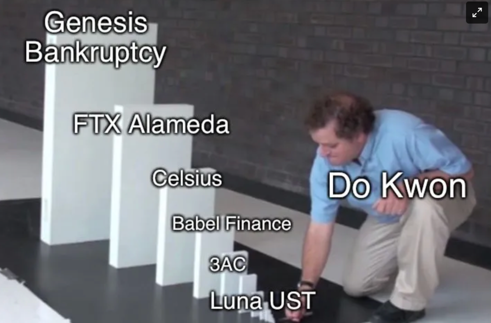
Failures of DCG and Genesis
Don't sleep with your own sister.
70% of lottery winners go broke within five years. You've heard the last one. People who got rich quickly without setbacks and hard work often lose it all. My father said, "Easy money is easily lost," and a wealthy friend who owns a family office said, "The first generation makes it, the second generation spends it, and the third generation blows it."
This is evident. Corrupt politicians in developing countries live lavishly, buying their third wives' fifth Hermès bag and celebrating New Year's at The Brando Resort. A successful businessperson from humble beginnings is more conservative with money. More so if they're atom-based, not bit-based. They value money.
Crypto can "feel" easy. I have nothing against capital market investing. The global financial system is shady, but that's another topic. The problem started when those who took advantage of easy money started affecting other businesses. VCs did minimal due diligence on FTX because they needed deal flow and returns for their LPs. Lenders did minimum diligence and underwrote ludicrous loans to 3AC because they needed revenue.
Alameda (hence FTX) and 3AC made "easy money" Genesis and DCG aren't. Their businesses are more conventional, but they underestimated how "easy money" can hurt them.
Genesis has been the victim of easy money hubris and insolvency, losing $1 billion+ to 3AC and $200M to FTX. We discuss the implications for the broader crypto market.
Here are the quick takeaways:
Genesis is one of the largest and most notable crypto lenders and prime brokerage firms.
DCG and Genesis have done related party transactions, which can be done right but is a bad practice.
Genesis owes DCG $1.5 billion+.
If DCG unwinds Grayscale's GBTC, $9-10 billion in BTC will hit the market.
DCG will survive Genesis.
What happened?
Let's recap the FTX shenanigan from two weeks ago. Shenanigans! Delphi's tweet sums up the craziness. Genesis has $175M in FTX.
Cred's timeline: I hate bad crisis management. Yes, admitting their balance sheet hole right away might've sparked more panic, and there's no easy way to convey your trouble, but no one ever learns.
By November 23, rumors circulated online that the problem could affect Genesis' parent company, DCG. To address this, Barry Silbert, Founder, and CEO of DCG released a statement to shareholders.
A few things are confirmed thanks to this statement.
DCG owes $1.5 billion+ to Genesis.
$500M is due in 6 months, and the rest is due in 2032 (yes, that’s not a typo).
Unless Barry raises new cash, his last-ditch efforts to repay the money will likely push the crypto market lower.
Half a year of GBTC fees is approximately $100M.
They can pay $500M with GBTC.
With profits, sell another port.
Genesis has hired a restructuring adviser, indicating it is in trouble.
Rehypothecation
Every crypto problem in the past year seems to be rehypothecation between related parties, excessive leverage, hubris, and the removal of the money printer. The Bankless guys provided a chart showing 2021 crypto yield.
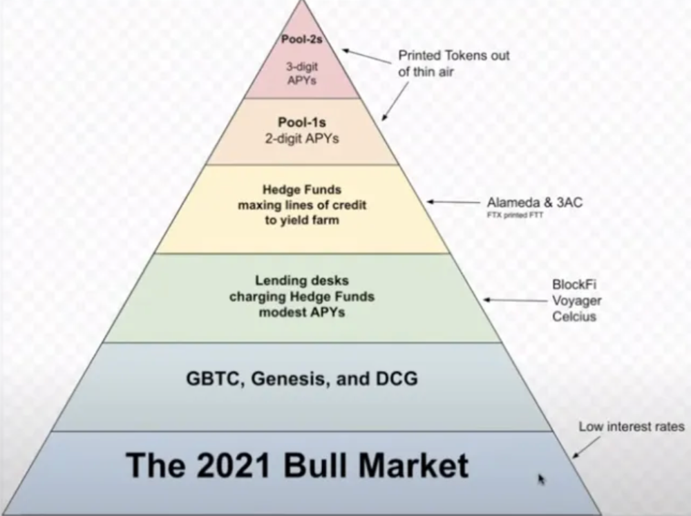
In June 2022, @DataFinnovation published a great investigation about 3AC and DCG. Here's a summary.
3AC borrowed BTC from Genesis and pledged it to create Grayscale's GBTC shares.
3AC uses GBTC to borrow more money from Genesis.
This lets 3AC leverage their capital.
3AC's strategy made sense because GBTC had a premium, creating "free money."
GBTC's discount and LUNA's implosion caused problems.
3AC lost its loan money in LUNA.
Margin called on 3ACs' GBTC collateral.
DCG bought GBTC to avoid a systemic collapse and a larger discount.
Genesis lost too much money because 3AC can't pay back its loan. DCG "saved" Genesis, but the FTX collapse hurt Genesis further, forcing DCG and Genesis to seek external funding.
bruh…
Learning Experience
Co-borrowing. Unnecessary rehypothecation. Extra space. Governance disaster. Greed, hubris. Crypto has repeatedly shown it can recreate traditional financial system disasters quickly. Working in crypto is one of the best ways to learn crazy financial tricks people will do for a quick buck much faster than if you dabble in traditional finance.
Moving Forward
I think the crypto industry needs to consider its future. This is especially true for professionals. I'm not trying to scare you. In 2018 and 2020, I had doubts. No doubts now. Detailing the crypto industry's potential outcomes helped me gain certainty and confidence in its future. This includes VCs' benefits and talking points during the bull market, as well as what would happen if government regulations became hostile, etc. Even if that happens, I'm certain. This is permanent. I may write a post about that soon.
Sincerely,
M.

Leon Ho
3 years ago
Digital Brainbuilding (Your Second Brain)

The human brain is amazing. As more scientists examine the brain, we learn how much it can store.
The human brain has 1 billion neurons, according to Scientific American. Each neuron creates 1,000 connections, totaling over a trillion. If each neuron could store one memory, we'd run out of room. [1]
What if you could store and access more info, freeing up brain space for problem-solving and creativity?
Build a second brain to keep up with rising knowledge (what I refer to as a Digital Brain). Effectively managing information entails realizing you can't recall everything.
Every action requires information. You need the correct information to learn a new skill, complete a project at work, or establish a business. You must manage information properly to advance your profession and improve your life.
How to construct a second brain to organize information and achieve goals.
What Is a Second Brain?
How often do you forget an article or book's key point? Have you ever wasted hours looking for a saved file?
If so, you're not alone. Information overload affects millions of individuals worldwide. Information overload drains mental resources and causes anxiety.
This is when the second brain comes in.
Building a second brain doesn't involve duplicating the human brain. Building a system that captures, organizes, retrieves, and archives ideas and thoughts. The second brain improves memory, organization, and recall.
Digital tools are preferable to analog for building a second brain.
Digital tools are portable and accessible. Due to these benefits, we'll focus on digital second-brain building.
Brainware
Digital Brains are external hard drives. It stores, organizes, and retrieves. This means improving your memory won't be difficult.
Memory has three components in computing:
Recording — storing the information
Organization — archiving it in a logical manner
Recall — retrieving it again when you need it
For example:
Due to rigorous security settings, many websites need you to create complicated passwords with special characters.
You must now memorize (Record), organize (Organize), and input this new password the next time you check in (Recall).
Even in this simple example, there are many pieces to remember. We can't recognize this new password with our usual patterns. If we don't use the password every day, we'll forget it. You'll type the wrong password when you try to remember it.
It's common. Is it because the information is complicated? Nope. Passwords are basically letters, numbers, and symbols.
It happens because our brains aren't meant to memorize these. Digital Brains can do heavy lifting.
Why You Need a Digital Brain
Dual minds are best. Birth brain is limited.
The cerebral cortex has 125 trillion synapses, according to a Stanford Study. The human brain can hold 2.5 million terabytes of digital data. [2]
Building a second brain improves learning and memory.
Learn and store information effectively
Faster information recall
Organize information to see connections and patterns
Build a Digital Brain to learn more and reach your goals faster. Building a second brain requires time and work, but you'll have more time for vital undertakings.
Why you need a Digital Brain:
1. Use Brainpower Effectively
Your brain has boundaries, like any organ. This is true while solving a complex question or activity. If you can't focus on a work project, you won't finish it on time.
Second brain reduces distractions. A robust structure helps you handle complicated challenges quickly and stay on track. Without distractions, it's easy to focus on vital activities.
2. Staying Organized
Professional and personal duties must be balanced. With so much to do, it's easy to neglect crucial duties. This is especially true for skill-building. Digital Brain will keep you organized and stress-free.
Life success requires action. Organized people get things done. Organizing your information will give you time for crucial tasks.
You'll finish projects faster with good materials and methods. As you succeed, you'll gain creative confidence. You can then tackle greater jobs.
3. Creativity Process
Creativity drives today's world. Creativity is mysterious and surprising for millions worldwide. Immersing yourself in others' associations, triggers, thoughts, and ideas can generate inspiration and creativity.
Building a second brain is crucial to establishing your creative process and building habits that will help you reach your goals. Creativity doesn't require perfection or overthinking.
4. Transforming Your Knowledge Into Opportunities
This is the age of entrepreneurship. Today, you can publish online, build an audience, and make money.
Whether it's a business or hobby, you'll have several job alternatives. Knowledge can boost your economy with ideas and insights.
5. Improving Thinking and Uncovering Connections
Modern career success depends on how you think. Instead of overthinking or perfecting, collect the best images, stories, metaphors, anecdotes, and observations.
This will increase your creativity and reveal connections. Increasing your imagination can help you achieve your goals, according to research. [3]
Your ability to recognize trends will help you stay ahead of the pack.
6. Credibility for a New Job or Business
Your main asset is experience-based expertise. Others won't be able to learn without your help. Technology makes knowledge tangible.
This lets you use your time as you choose while helping others. Changing professions or establishing a new business become learning opportunities when you have a Digital Brain.
7. Using Learning Resources
Millions of people use internet learning materials to improve their lives. Online resources abound. These include books, forums, podcasts, articles, and webinars.
These resources are mostly free or inexpensive. Organizing your knowledge can save you time and money. Building a Digital Brain helps you learn faster. You'll make rapid progress by enjoying learning.
How does a second brain feel?
Digital Brain has helped me arrange my job and family life for years.
No need to remember 1001 passwords. I never forget anything on my wife's grocery lists. Never miss a meeting. I can access essential information and papers anytime, anywhere.
Delegating memory to a second brain reduces tension and anxiety because you'll know what to do with every piece of information.
No information will be forgotten, boosting your confidence. Better manage your fears and concerns by writing them down and establishing a strategy. You'll understand the plethora of daily information and have a clear head.
How to Develop Your Digital Brain (Your Second Brain)
It's cheap but requires work.
Digital Brain development requires:
Recording — storing the information
Organization — archiving it in a logical manner
Recall — retrieving it again when you need it
1. Decide what information matters before recording.
To succeed in today's environment, you must manage massive amounts of data. Articles, books, webinars, podcasts, emails, and texts provide value. Remembering everything is impossible and overwhelming.
What information do you need to achieve your goals?
You must consolidate ideas and create a strategy to reach your aims. Your biological brain can imagine and create with a Digital Brain.
2. Use the Right Tool
We usually record information without any preparation - we brainstorm in a word processor, email ourselves a message, or take notes while reading.
This information isn't used. You must store information in a central location.
Different information needs different instruments.
Evernote is a top note-taking program. Audio clips, Slack chats, PDFs, text notes, photos, scanned handwritten pages, emails, and webpages can be added.
Pocket is a great software for saving and organizing content. Images, videos, and text can be sorted. Web-optimized design
Calendar apps help you manage your time and enhance your productivity by reminding you of your most important tasks. Calendar apps flourish. The best calendar apps are easy to use, have many features, and work across devices. These calendars include Google, Apple, and Outlook.
To-do list/checklist apps are useful for managing tasks. Easy-to-use, versatility, budget, and cross-platform compatibility are important when picking to-do list apps. Google Keep, Google Tasks, and Apple Notes are good to-do apps.
3. Organize data for easy retrieval
How should you organize collected data?
When you collect and organize data, you'll see connections. An article about networking can assist you comprehend web marketing. Saved business cards can help you find new clients.
Choosing the correct tools helps organize data. Here are some tools selection criteria:
Can the tool sync across devices?
Personal or team?
Has a search function for easy information retrieval?
Does it provide easy data categorization?
Can users create lists or collections?
Does it offer easy idea-information connections?
Does it mind map and visually organize thoughts?
Conclusion
Building a Digital Brain (second brain) helps us save information, think creatively, and implement ideas. Your second brain is a biological extension. It prevents amnesia, allowing you to tackle bigger creative difficulties.
People who love learning often consume information without using it. Every day, they postpone life-improving experiences until they're forgotten. Useful information becomes strength.
Reference
[1] ^ Scientific American: What Is the Memory Capacity of the Human Brain?
[2] ^ Clinical Neurology Specialists: What is the Memory Capacity of a Human Brain?
[3] ^ National Library of Medicine: Imagining Success: Multiple Achievement Goals and the Effectiveness of Imagery